Persistence
Data artifacts due to persistence can affect all JWST observations. This article describes the methods available to correct for these artifacts.
On this page
Extremely bright sources, and some cosmic rays, can cause afterglow artifacts that persist for hundreds to thousands of seconds after the original charge is deposited on the detector. The detailed physics of this charge capture varies between the near-IR and mid-IR detectors, but the typical manifestation is as an exponentially decaying signal affecting pixels that received a large amount of charge. This residual signal is typically positive, but for the mid-IR detectors can in some cases be negative due to changes in the effective sensitivity of the pixel. The strongest persistence is produced when pixels reach full-well saturation (roughly 55,000 DN, varying for different detectors), but fainter artifacts can be produced even when the detector ramps do not reach saturation.
The timescale for these artifacts can vary from pixel to pixel, and each pixel may have multiple different decay timescales according to the various charge traps that were filled by photoelectrons. Likewise, the effective persistence timescale can vary based on the degree of saturation, the length of time spent at saturation, the number of read-resets prior to the next exposure, and the incident background signal in later exposures. For example, persistence decays to 0.01% of the original signal in about 15 minutes for MIRI and is undetectable after about 30 minutes (see detailed discussion by Dicken et al. 2024). Persistence timescales and characteristics in the NIRCam NIR detectors is described by NIRCam Persistence, along with a description of operational strategies used to mitigate the impact of objects that pose a significant persistence risk.
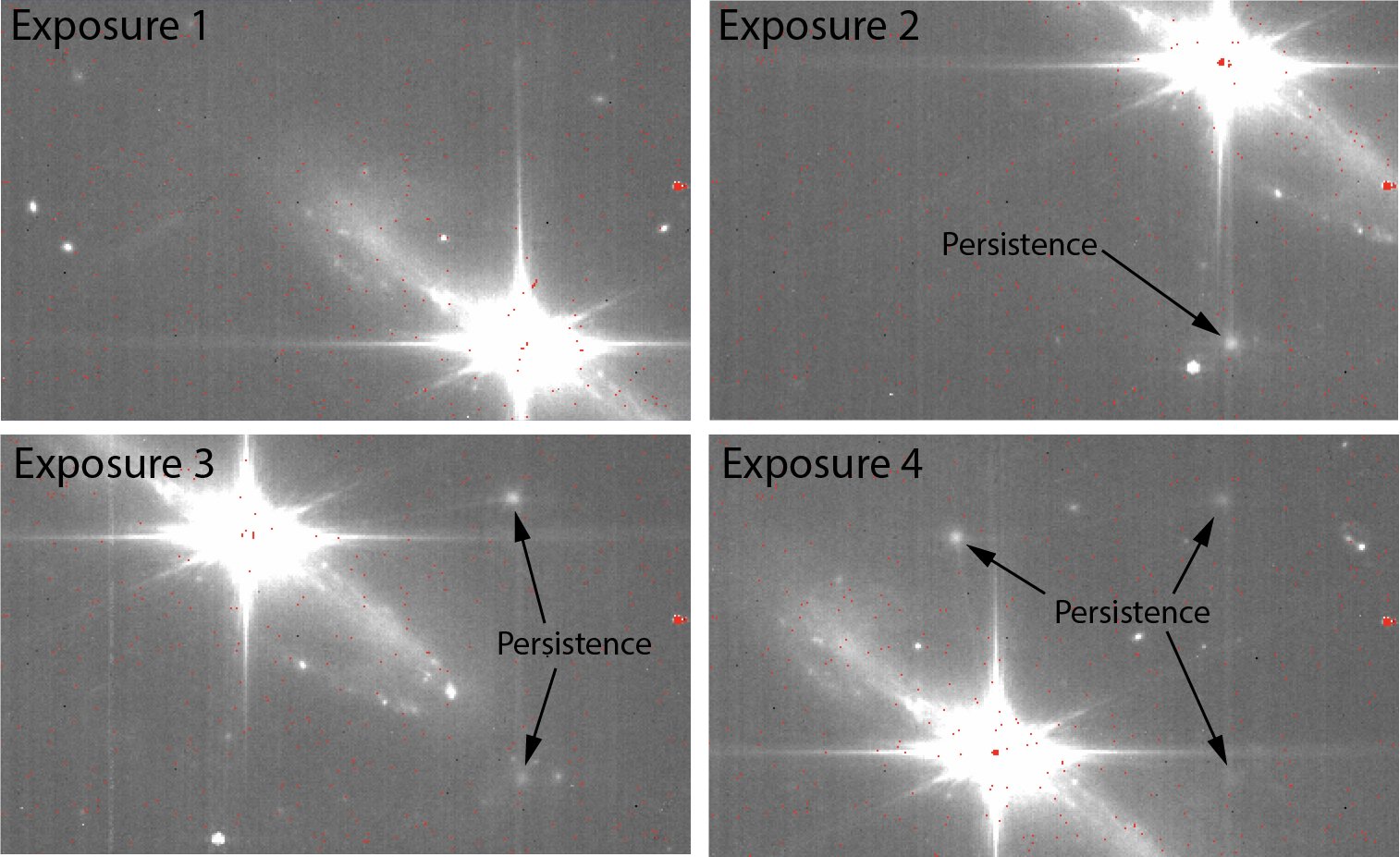
Figure 1. Illustration of persistence
Click on the figure for a larger view.
Illustration of persistence in MIRI F560W imaging observations of a bright AGN embedded in galaxy NGC 6552 (JWST program ID 1039). Persistence artifacts are visible in each exposure in the pixels at the center of the bright AGN in prior exposures and slowly decay over time. Red regions represent pixels with NaN values that are masked as DO_NOT_USE in the data quality array. In this example, exposures are approximately 3 minutes apart.
Pipeline Persistence step
As of pipeline build 13.0, a new pipeline step has been developed to help flag and mask pixels likely to be affected by persistence. This step replaces the persistence step in previous pipeline versions, which created unused "trapsfilled.fits" files that modeled the number of charge traps filled at the end of each integration but was not generally useful for flagging persistence.
The new persistence step is located within the calwebb_detector1 pipeline immediately prior to the ramp_fit step. This step looks for all pixels that reached saturation (or a user-defined DN threshold) in any group, and flags all later groups within a characteristic persistence time window with the PERSISTENCE data quality flag. This persistence information is also saved to an intermediate ASDF-format file which can be read during calwebb_detector1 processing of later exposures and used to pass persistence information between exposures.
As described by ReadTheDocs, the persistence step is governed by a few key parameters:
- persistence.skip: By default, the persistence step is skipped by the jwst pipeline. In order to run the step, users must set skip=False.
- persistence.save_persistence: Users should provide a filename (e.g., 'persistence.asdf') to use to store information about saturation events and pass this information to the next exposure.
- persistence.persistence_array_file: The file containing persistence information that was recorded when processing previous exposures. Typically, this should be the same as the ASDF filename given to the save_persistence parameter. However, they can be different if users wish to have finer control over the flagging (see discussion below).
- persistence.persistence_time: The length of time in seconds to use for the persistence flagging window. This will need to be tuned by hand to match the persistence observed in a given data set, but 900 seconds will often be a reasonable starting estimate.
- persistence.dn_threshold: An optional DN threshold above which persistence flagging should be performed. This allows customization to control flagging for nearly-saturating pixels.
- persistence.persistence_dnu: By default, pixels that are expected to be affected by persistence only have the 'PERSISTENCE' flag set in the data quality array. This is an informational bit flag only, and does not affect data processing. If persistence_dnu=True, such pixels will also be flagged with the DO_NOT_USE bit ensuring that they are rejected by the jwst pipeline and not used in ramp fitting.
Since this step is new in build 13.0, it is currently skipped by default and no characteristic persistence timescales have been provided. Baseline timescales for each instrument will be added in a future build, although users wishing to take advantage of persistence flagging must reprocess their data to do so. Note that exposures must be processed in time order by the calwebb_detector1 pipeline in order for persistence information to be passed effectively between exposures. Interleaved detectors however, are ok—the ASDF file will save information for each detector (e.g., NRCA1 vs NRCA2) separately.
If using the JWST Pipeline Notebooks to reprocess data for instance, the calwebb_detector1 dictionary might be configured as follows:
det1dict['persistence']['skip']=False
det1dict['persistence']['persistence_time']=900
det1dict['persistence']['save_persistence']='persist.asdf'
det1dict['persistence']['persistence_dnu']=True
det1dict['persistence']['save_results']=True
det1dict['persistence']['persistence_array_file']='persist.asdf'
det1dict['persistence']['dn_threshold']=40000
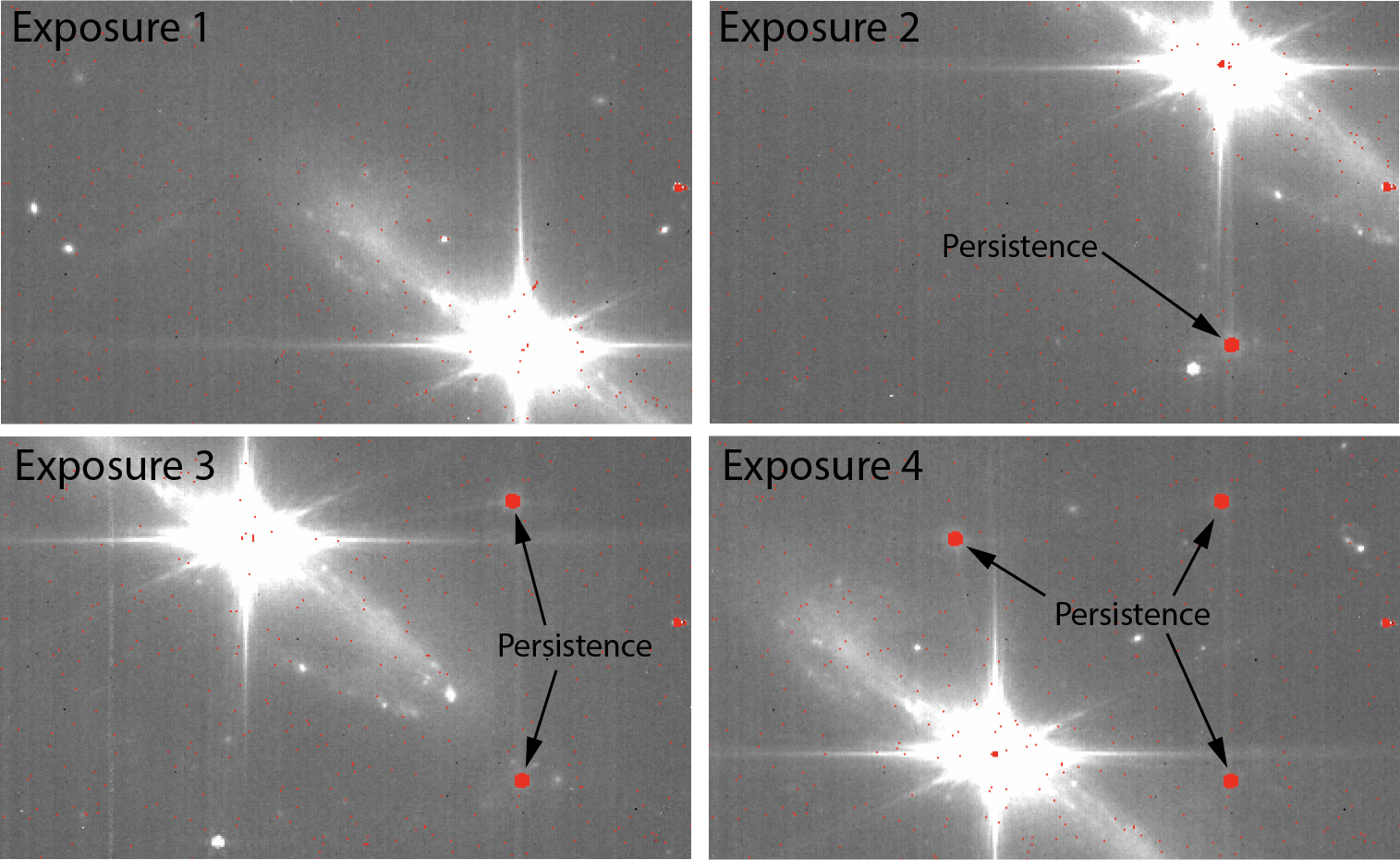
Figure 2 below shows the results of applying these parameters to reprocessing of the MIRI imaging example from Figure 1 above; persistence artifacts are now mostly masked in subsequent exposures.
Figure 2. Illustration of persistence flagging
Click on the figure for a larger view.
As Figure 1, but with pipeline persistence flagging applied. Note that pixels affected by persistence are now populated by NaNs (red regions) and masked as DO_NOT_USE in the data quality array.
Who should use the persistence step?
In most cases, it will be unnecessary for users to run the persistence step. Typically any persistence is not scientifically significant, and in many cases with mild persistence in imaging modes the outlier detection that occurs prior to combining dithered data can detect and reject persistence artifacts with no special intervention. Likewise, observatory scheduling is designed to prevent the worst cases of persistence, such as from bright solar system observations impacting later deep field programs.
Two typical cases exist in which the persistence step may be of use to science users:
- Observations with persistence in which the artifacts are not sufficiently rejected by the standard outlier detection routine (or in which data are not being combined across dithers).
- Extremely deep (often spectroscopic) observations in which cosmic rays can cause persistence within and between exposures.
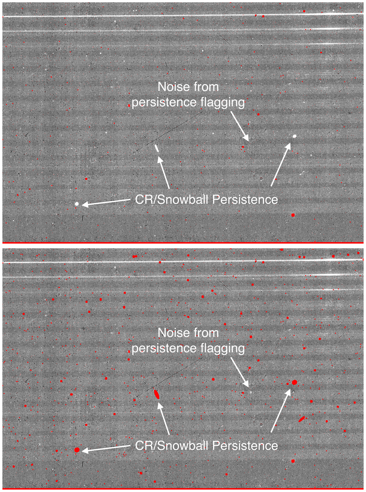
Figure 3 below shows an example of a deep NIRSpec IFU exposure that is contaminated by the persistence from many cosmic rays/snowballs, and how persistence flagging can aid in masking this contamination (using the parameter configuration defined above and a longer persistence.persistence_time = 3600).
The decision whether or not to run the persistence step, and how to configure it, is highly science-case and observing-mode dependent. The persistence step only knows where persistence has the potential to occur, and not whether it will be scientifically significant enough to warrant rejecting the affected pixels. If the pixels containing a saturated source in one exposure falls on a faint region of scientific interest in the second exposure, artifacts may be relevant. However, if those pixels land on a bright target in the second exposure small artifacts may be irrelevant. Some spectroscopic modes with limited dithering (e.g., MIRI MRS) may therefore need to customize how the persistence flags are being interpreted in order to avoid over-rejection of bright pixels for which persistence is present but unimportant.
Figure 3. Illustration of flagging persistence from cosmic rays and snowballs in a deep exposure
Click on the figure for a larger view.
Illustration of persistence and persistence flagging in a deep NIRSpec IFU observations of a high-z AGN, VDESJ0020-3653 (JWST program ID 1222). Sky illumination of the IFU slices can be seen as horizontal bands, with slices at the top of the image containing illumination from the AGN. Persistence artifacts from cosmic rays (CR) and snowballs that occurred in prior exposures are visible across the image. The image blinks between the "rate" image from default pipeline processing and produced re-processing the data with the persistence step to flag pixels affected by persistence as DO_NOT_USE (red pixels) with persistence.persistence_time = 3600. Note that flagging persistence pixels with DO_NOT_USE is done group-by-group, and can represent a tradeoff in data quality. While flagging can remove known persistence artifacts, in some cases it can also cause artifacts due to noisy "rate" measurements from severely truncated ramps as highlighted in the above example.
References
Dicken, D., et al. 2024, A&A, 689, A5
JWST MIRI flight performance: Imaging