NIRCam Short Wavelength Grism Time Series
JWST NIRCam's short wavelength grism time-series observing mode uses the Dispersed Hartmann Sensor (DHS) to perform rapid spectroscopic (R ~ 300) monitoring of bright, time-variable sources at 0.6–2.3 µm. It was added to the NIRCam grism time-series APT template for Cycle 4, but has its own calculation type in the JWST ETC.
On this page
See also: NIRCam Grism Time-Series APT Template, NIRCam Short Wavelength Grism Time Series Observing Strategies and NIRCam Grism Time Series
The NIRCam DHS was designed to support phasing of the JWST mirror segments during commissioning, but is now available in the NIRCam Grism Time-Series APT Template to provide point source spectroscopy in the short wavelength (SW) channel. It can only be paired with the long wavelength (LW) grism, and in that combination provides wavelength coverage within the 0.6–5.0 µm range.
Words in bold are GUI menus/
panels or data software packages;
bold italics are buttons in GUI
tools or package parameters.
More information about multistripe subarrays is available at NIRCam Multistripe Subarrays for Grism Time Series Spectroscopy. The GDHS0 element, which disperses spectra along detector rows, is available for science. The GDHS60 element disperses at an oblique angle across the detectors, and is reserved for engineering purposes. Through the remainder of this article "DHS" implies the GDHS0 element in the NIRCam module A short wavelength channel. Science applications of the DHS for transit spectroscopy were described by Schlawin et al. (2017).
Due to the complexities of new detector readout operations and limited time to obtain on-sky calibration data prior to Cycle 4 observations, the accuracy of the JWST ETC for the short wavelength grism time-series calculations may not meet the 10% accuracy requirement. As a result, this capability is being offered on a shared-risk basis in Cycle 4. Calibration observations were/will be obtained and used to improve the accuracy of the ETC and the pipeline during and after Cycle 3.
Optical properties of the Dispersed Hartmann Sensor (DHS) pupil element and its grisms
The DHS pupil wheel element is composed of 10 separate grisms that occupy rectangular sub-apertures. Each grism includes a wedge in the cross-dispersion direction such that 10 spectra are produced, and are well separated in the cross-dispersion direction. The properties of the grisms and the spectra they produce are summarized below. A new detector readout mode, multistripe subarrays, has been implemented to optimally sample the individual spectra while skipping over portions of the detector devoid of spectral signal.
DHS pupil sub-aperture alignment to the primary mirror pupil
The alignment of the DHS sub-apertures has been adjusted such that the dispersion direction is parallel to detector rows of the NIRCam short wavelength detectors in module A, and is shown in Figure 1. This alignment allows narrow subarrays with short frame times to be used, which is desirable for observations of very bright host stars of transiting exoplanets. The location of the DHS sub-apertures relative to the JWST primary mirror pupil is shown below. Because the pupil wheel rotational position aligning spectra with rows is different from that used for commissioning of the primary mirror, overlap of some of the sub-apertures is less than optimal. Both the throughput and the quality of the PSF is degraded, particularly for sub-apertures 1 and 6. The highest throughput sub-apertures are 4 and 7, which also have the sharpest PSFs. Of the remaining sub-apertures, throughput and PSF quality don't vary greatly, with sub-aperture 9 being somewhat worse.
Figure 1. An RGB image overlay of of the JWST primary mirror (green), NIRCam DHS apertures (blue), and STPSF DHS pupil mask (red)

This image shows the alignment of the 10 sub-apertures of the NIRCam DHS grism element, JWST primary mirror, and the STPSF (formerly WebbPSF) pupil mask for the DHS. The DHS sub-apertures appear yellow, the primary mirror light green, and the STPSF sub-apertures red in this color projection. These data were used to refine the sub-aperture locations of the STPSF pupil mask prior to generating the DHS PSFs needed for the ETC. This alignment produces DHS spectra that are parallel to pixel rows on the NIRCam detectors, and differs significantly from that used for coarse phasing of the JWST primary during commissioning. Sub-apertures 1 and 6 are not used for science, while options in APT and the ETC allow use of the spectra produced by aperture combinations: 2-spectra (4 & 7), 4-spectra (2, 4, 7, 8), and 8-spectra (2, 3, 4, 5, 7, 8, 9, 10). "Pond-ring" features in the image above are a known feature of the NIRCam pupil imaging lens (PIL) and do not impact spectral data. Numerous micro-meteoroid strikes can also be seen on the primary. Data are from program 4510, observation 4.
Table 1a. Fractional area of the DHS sub-apertures relative to the area of the primary mirror
| DHS sub-aperture | 2 | 3 | 4 | 5 | 7 | 8 | 9 | 10 | Total |
| Fractional Area (%) | 3.12 | 3.13 | 3.86 | 2.67 | 3.94 | 3.53 | 2.78 | 2.75 | 25.8 |
Sub-aperture (spectrum) combinations
Users can choose to simultaneously collect spectra from 2, 4 or 8 of the DHS sub-apertures (also simultaneously with the long wavelength grism spectrum). The sub-apertures included in those combinations and the combined throughput is summarized in Table 1b.
Table 1b. DHS sub-apertures included in the 2-Spectra, 4-Spectra and 8-Spectra subarray
| Subarray selection determines the # of spectra selected | 2 spectra | 4 spectra | 8 spectra |
| DHS sub-apertures included | 4, 7 | 2, 4, 7, 8 | 2, 3, 4, 5, 7, 8, 9, 10 |
\Sigma(Fractional aperture throughput) (%) | 7.8 | 14.5 | 25.8 |
Spectra produced by the DHS grisms
Example DHS spectra of a single point-source target are shown in Figure 2. Data were taken using the FULL subarray and were used to determine the substripe locations to be used for the multistripe subarrays. The spectra fall on the lower (-V3) portions of detectors A2 and A4, and the upper (+V3) portions of detectors A1 and A3 (see Figure 9 below and NIRCam Field of View). Users have some flexibility to select which spectra to collect: the 2 brightest, the 4 brightest or the 8 brightest. Spectra from DHS sub-apertures 1 and 6 have very much lower throughput (see Figure 1, above), much broader point spread and line spread functions, and significantly lower resolving power than the other 8 sub-apertures, and data for them are not collected (and in fact fall in the SW detector gap, by design). Figure 3 shows data collected using the actual multistripe subarrays.
Figure 2. Full frame images of spectra produced by the LW GRISMR and SW DHS0 elements from a calibration observation

Above: Cropped image of a LW grism spectrum acquired at the F322W2 field point through filter F322W2.
The star symbol shows the target location in direct images.

Above: Cropped image of DHS + F150W2 spectra on the 4 SW detectors taken simultaneously with the LW spectrum above. (The "F322W2" labels on these SW images convey the along-dispersion field point used, which is determined by the LW filter chosen for the observation.)
The rectangles show the size and position of the SUB164S4_8-SPECTRA subarrays. Orange rectangles below show the region of contamination by 2nd-order light.

Above: Cropped image of a LW grism spectrum acquired at the F444W field point through filter F444W. The star symbol shows the target location in direct images.

Above: Cropped image of DHS + F150W2 spectra on the 4 SW detectors taken simultaneously with the LW spectrum above. (The "F444W" labels on these SW images convey the along-dispersion field point used, which is determined by the LW filter chosen for the observation.)
The rectangles show the size and position of the SUB164S4_8-SPECTRA subarrays (which actually extend across the full width of the A3 & A4 detectors).
Click on the figures for a larger view.
Long wavelength GRISMR spectra and short wavelength DHS0 spectra acquired simultaneously in program 4453. Data were acquired using the FULL subarray on all detectors, but these images have been cropped to show just the regions near the spectral traces. The top two panels show the single LW grism spectrum taken through the F322W2 filter, and the corresponding 8 spectra from the DHS with the F150W2 filter on the SW detectors. The bottom two panels show the single LW grism spectrum taken through the F444W filter, and the corresponding 8 spectra from the DHS with the F150W2 filter on the SW detectors. Star symbols on the LW images show the location of the direct image if the GRISMR element were not in the beam (there is a small vertical offset due to the grism). On the SW channel, the target is located in the horizontal gap between the A2 + A4 detectors and the A1 + A3 detectors. The spectra from the DHS1 and DHS6 sub-apertures fall in that same gap.
Figure 3. Multistripe subarray images of DHS and LW Grism spectra of a calibration star obtained on-orbit
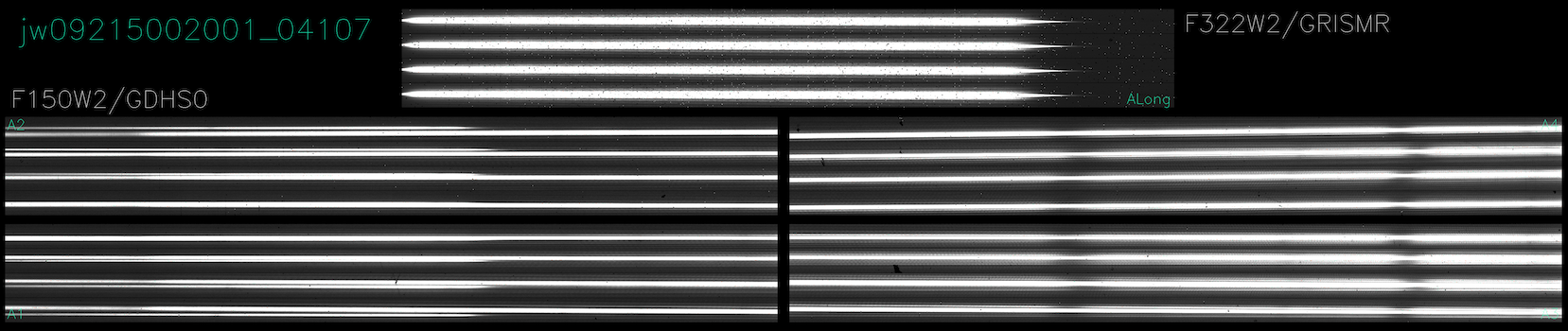
Above: The figure shows data taken using the F322W2 + GRISMR combination in the LW channel and F150W2 + DHS0 in the SW channel.
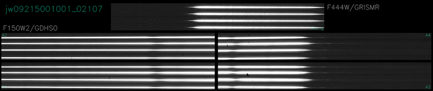
Above: The figure above data taken using the F444W + GRISMR combination in the LW channel and F150W2 + DHS0 in the SW channel.
Click on the figures for a larger view.
Two 5-panel composite figures showing the multistripe subarray images from the LW detector (top) and the 4 SW detectors (A2, A4, A3, A1, clockwise starting from upper left). These data were taken with the SUB260S4_8Spectra subarray which captures 4 spectra from individual DHS sub-apertures on the SW detectors while sampling the single LW GRISM spectrum on the LW detector 4 times. Data are from program 9215 Observation 1, which acquired spectra through all filter combinations in the Grism Time Series template.
DHS point spread and line spread functions
Because the DHS sub-apertures are much smaller than the primary mirror aperture, and are oblong (see Figure 4), the monochromatic PSFs from them are very different from the normal JWST PSFs. In particular they are very elongated in the dispersion direction. The width of the monochromatic PSF in the dispersion direction is the line spread function (LSF) and determines the resolving power.
Figure 4. Example monochromatic PSFs for DHS sub-apertures 4 and 7

Click on the figure for a larger view.
STPSF monochromatic PSFs at 1.05 (top row) and 2.07 µm (bottom row) for the DHS, displayed on a log scale. The horizontal axis is the dispersion direction. The left and middle columns are for DHS0 sub-apertures 4 & 7 respectively. The right column is the co-addition of the two sub-aperture PSFs, and is used in the ETC if users pick the 2 spectra option. The native pixels are oversampled by a factor of 3 in these images, and correspond to 121 × 121 detector pixels (3.75'' × 0.035 µm). (The blue square surrounding the upper-right PSF has no significance, but will be familiar to users of the ds9 display package). With the transverse size of the individual DHS apertures being about 1/10 of the JWST primary mirror diameter, at 1 or 2 µm the LSF (i.e., the PSF in the dispersion direction), is about 10 or 20 NIRCam SW pixels. For reference, the short wavelength NIRCam imaging PSF FWHM is 2 pixels at 2 µm.
Dispersion and resolving power
The DHS grisms have constant dispersion over the wavelength range of interest (0.6–2.2 µm). The resolving power is entirely controlled by the line spread function at all wavelengths, and is also constant vs. wavelength. The values are given below for 1st and 2nd order. The grisms have significantly higher throughput below 0.9 µm in 2nd order than in 1st, so 2nd order spectra for the shortest filters (see Table 3) will be most useful for science. For the F150W2 filter, the 2nd order DHS spectra at wavelengths 1.01–1.15 µm overlap the 1st order spectrum starting at 2.02 µm. While that filter has good transmission out to 2.3 µm, observers should consider using the F200W filter if they are particularly interested in wavelengths 2.0–2.3 µm. Contamination by 2nd order spectra is only an issue for the F150W2 filter.
Table 2. DHS dispersion and resolving power
| Dispersion (nm/pixel) | Resolving Power (\lambda / \delta \lambda) | ||
| 1st Order | 2nd Order | 1st Order | 2nd Order |
| 0.290 | 0.145 | 300 | 600 |
Throughput
The DHS grisms have an anti-reflection coating that has very high transmission beyond 1 µm, and a steeply declining transmission below that. The grism blaze function also results in lower throughput below about 1.2 µm, so the overall throughput in 1st order is low at the shortest NIRCam wavelengths. The grisms are more efficient in 2nd order below about 0.9 µm, as can be seen in Figure 5.
Figure 5. Throughput of the DHS grisms

Click on the figure for a larger view.
Throughput of the DHS grisms in 1st and 2nd order. The throughput includes the anti-reflection coating transmission and the grism blaze function. The yellow shaded area below 0.8 μm indicates that the DHS performance in this spectral region has not been fully characterized yet, but is expected to improve during Cycle 3 as more calibration data are taken. The throughput is multiplied by the sub-aperture fractional overlap with the OTE pupil (see Table 1b) in order to compute throughput for each spectrum.
Allowed filters
The DHS can be paired with the filters given in Table 3. The F150W2 filter offers the largest grasp (1.01–2.38 μm), but is also more susceptible to contamination by nearby sources than the narrower filters. Moreover, longward of 2 μm the spectra are contaminated by 2nd order light from 1.01–1.19 μm, so observers should consider using F200W if they are interested in the 2–2.23 μm range. DHS throughput data at the wavelengths included in the F070W and F090W bandpasses is poorly characterized, but is significantly lower than for the longer filters, as shown in Figure 5.
Depending on the choice of LW filter, 2 possible field point locations along the spectral direction are possible, one corresponding to choosing long wavelength filters F277W/F356W/F322W2 and the other to choosing F444W (see NIRCam Grism Time Series). Selection of the long wavelength filter in APT controls the placement of the spectra in both the short and long wavelength channels: the location and spectral coverage in the short wavelength channel is entirely determined by the choice of long wavelength filter. Table 3 tabulates the spectral ranges on the SW detectors for each SW filter, spectral order, and choice of long wavelength filter. Cells marked in yellow correspond to low throughput combinations. The same ranges are visually displayed in Figure 6.
The exact wavelength ranges depend on the DHS sub-aperture. The values below are for the median dispersion solutions, but variations of ± ~0.01 µm occur due to slight differences in the location of the undeviated wavelength location on the detectors for the individual grisms. The undeviated wavelength is 1.36 μm.
Table 3. Wavelength coverage for the allowed SW grism spectroscopy blocking filters
DHS blocking filter | LW filter and spectral field point | Order | Wavelength range on A3/A4 (μm) | Wavelength range on A1/A2 (μm) |
|---|---|---|---|---|
F070W | F277W/F356W/F322W2 | 2nd | 0.62–0.78 | - |
F444W | 1st | 0.63–0.78† | - | |
| 2nd | 0.64–0.78 | |||
F090W | F277W/F356W/F322W2 | 2nd | 0.8–0.83 | 0.86–1.00 |
F444W | 1st | 0.8–1.00† | - | |
| 2nd | 0.8–0.94 | |||
F115W | F277W/F356W/F322W2 | 1st | 1.07–1.28 | - |
| 2nd | - | 1.01–1.15†† | ||
F444W | 1st | 1.01–1.23 | ||
F150W2 | F277W/F356W/F322W2 | 1st | 1.07–1.66 | 1.71–2.01* |
F444W | 1st | 1.01–1.23 | 1.28–1.89 | |
F200W | F277W/F356W/F322W2 | 1st | - | 1.76–2.23 |
F444W | 1st | - | 1.76–1.89 |
† The DHS has low throughput shortward of 1 μm for 1st order spectra.
†† The DHS has low throughput longward of 1 μm for 2nd order spectra.
* The 2.01 μm cutoff is due to 1st and 2nd order overlap, although nominally the spectra extend to 2.25 μm.
Figure 6. Modeled DHS spectra locations and wavelength coverage for each blocking filter

Click on the figure for a larger view.
Wavelength coverage from Table 3 for the available DHS blocking filters. The vertical black lines represent the horizontal extent of the NIRCam SW detectors (A1 & A2 at left, A3 & A4 at right), with the science X coordinate increasing to the right, while wavelength increases to the left. The vertical axis is arbitrary. First order spectra footprints are show in blue, while second order are in orange. The top and bottom panels are for the along-dispersion field points, as determined by the filter choice on the LW channel. The gray vertical dashed lines represent the position of the undeflected wavelength (1.36 or 0.68 μm in 1st and 2nd order, respectively), and also the position of a direct image at either the F322W2 or F444W field point.
Saturation and sensitivity
Because the DHS sub-apertures sample such small fractions of the primary mirror (see Table 1), saturation limits are relatively high and sensitivity relatively low compared to the long wavelength grism time-series values.
Saturation limit varies by sub-aperture, with #7 having the highest throughput. Depending on how many sub-aperture spectra the user has chosen to collect (2, 4 or 8), saturation of the sub-aperture 7 spectrum may or may not be a particular concern. Figure 7 shows the saturation limit for sub-aperture 7, thus providing the most conservative estimate. Figure 8 shows the predicted sensitivity for cases where 2, 4 or 8 of the sub-aperture spectra have been co-added.
Figure 7. Saturation limits for the DHS vs. stellar spectral type and blocking filter

Click on the figure for a larger view.
Saturation limits as a function of equivalent K magnitude (left axis) and flux density (right axis) for A0V, G2V and M2V stellar types (colored lines), and in the F070W, F090W, F150W2, F200W filters (note that F070W and F090W are used in 2nd order, while F150W2 and F200W are used in 1st). Saturation limits for the F115W and F150W filters are similar to those shown for F150W2 within their respective bandpasses. The saturation limit as a function of flux density is given by the black lines. The saturation limits are much brighter for the DHS than for the long wavelength grism: typically it is the long wavelength grism that will restrict the integration time used for a given observation. The gray shaded area below 0.8 μm indicates that the DHS performance in this spectral region has not been fully characterized yet. Note that while F150W2 has good transmission beyond 2.0 μm, 1st and 2nd order spectra overlap there. Observers should consider using the F200W filter for that region.
Figure 8. Sensitivity for the DHS vs subarray size and blocking filter

Click on the figure for a larger view.
Sensitivity of the DHS vs wavelength for the 2, 4 and 8 spectra cases (STRIPE1, 2 and 4 subarrays, respectively) in the F070W, F090W and F150W2 filters. Note that this has been computed per spectral pixel, rather than per resolution element. The spectral resolution is determined by the size of the LSF, which changes linearly with wavelength (i.e., the resolving power is constant), and goes from 10 pixels at 1 μm to 20 pixels at 2 μm. The measurement time of 100 s and the SNR of 100 have been chosen as representative of the typical usage of this mode for transiting exoplanet studies. Sensitivities for F070W and F090W are for 2nd-order spectra, F150W2 values are for the 1st order spectrum, and all are for a single 100 s integration. The gray shaded area below 0.8 μm indicates that the DHS performance in this spectral region has not been fully characterized yet. Sensitivity for the SUB260S4_8-SPECTRA subarray is very close to that of SUB164S4_8-SPECTRA. Observers should use the ETC to evaluate SNR for their particular targets.
Subarrays for DHS time-series spectroscopy
The subarrays used to read out pixels associated with the individual DHS spectra (see Figure 1) are part of a new capability developed for Cycle 4, named multistripe. In summary, a multistripe subarray consists of multiple stripes (contiguous rows of pixels). These "substripes" need not be contiguous on the detector, and the placement of the substripes is configurable within certain limits. Users are referred to the article NIRCam Multistripe Subarrays for Grism Time Series Spectroscopy for additional details about the capability.
For DHS grism time-series observations, 4 sizes of multistripe subarrays are available, providing flexibility in terms of the frame time and the number of spectra read out. Each multistripe subarray includes 1 row of reference pixels read out once for each substripe (see Figure 3 at the Multistripe Subarrays article linked above). The complete set of substripes, including the reference pixel rows, comprises a subarray frame.
When SW Channel Mode is set to GRISM in the NIRCam Grism Time Series APT template, the target is positioned such that 4 of the DHS spectra fall on detectors A1 and A3 while the other 4 spectra fall on A2 and A4. The same subarray size must be used in both the short and long wavelength channel of NIRCam. However, there is only one spectrum in the LW channel. The multistripe capability allows a single substripe to be read out repeatedly during the subarray frame time. That is done on the LW channel, providing multiple samples of the LW spectrum within the subarray frame time, while spatially separated stripes are being sampled on the SW detectors.
Figure 9 is a schematic showing the locations of the DHS spectra in the SW channel and the LW grism spectrum in the LW channel (see also Figure 2). While 2, 4 or 8 of the DHS spectra are being read, the corresponding LW grism substripe is read 1, 2 or 4 times more frequently. For targets where photon statistics dominate, the oversampling of the LW spectrum has a tiny effect on the SNR of that spectrum, but there are potential benefits in terms of the LW saturation limit. While the ETC does not currently capture those benefits, the stage 0 and stage 1 data products include the extra LW reads.
Figure 9. Schematic showing the locations of the SW DHS spectra and the LW spectrum

Click on the figure for a larger view.
Blue lines in the left half of the figure represent the DHS spectra projected onto the SW detectors. Combinations of 2, 4 or 8 spectra are supported. While those spectra are being read in the SW channel, the LW multistripe subarray repeatedly samples just the LW spectrum (represented by the red line at right). Approximate locations of the direct images of the target, and the field points used for the F444W and F322W2 filters in the LW channel, are shown by the yellow circles (note that the two other available filter choices on the LW channel, F277W and F356W correspond to a spectral placement identical to the F322W2 case). Red squares are the origin of the detector readout coordinate system. Spectra from DHS sub-apertures 1 and 6 are of significantly lower quality, and are intentionally placed in the gap between the SW detectors. In this way, the maximum number of higher throughput SW DHS spectra can be read out simultaneously on 4 detectors while keeping frame and integration times short on the LW.
Table 4 summarizes the multistripe subarrays available for the SW DHS grism mode, and the corresponding oversampling that occurs in the LW channel.
Table 4. DHS time series multistripe subarray parameters
| # Reads per spectrum per tFrame | ||||||||
Subarray Name | # Substripes per SCA | # Spectra | Rows per substripe* | Frame time (tFrame) | Stripe time† | SW (DHS) | LW (Grism) | DHS spectra included |
SUB41S1_2-SPECTRA | 1 | 2 | 41 | 0.22009 | 0.21484 | 1 | 1 | 4, 7 |
SUB82S2_4-SPECTRA | 2 | 4 | 41 | 0.43493 | 1 | 2 | 2, 4, 7, 8 | |
| SUB164S4_8-SPECTRA | 4 | 8 | 41 | 0.86461 | 1 | 4 | 2, 3, 4, 5 7, 8, 9, 10 | |
| SUB260S4_8-SPECTRA | 4 | 8 | 65 | 1.36765 | 0.34060 | 1 | 4 | |
* Each substripe consists of Reads1 = 1 row of reference pixels plus Reads2 rows (either 40 or 64) of light sensitive pixels. The subarray frame contains (# Substripes per SCA) * (Rows per substripe) total rows.
† The time to read "Rows per substripe" rows of pixels. See also the "Multistripe timing equations" section in NIRCam Multistripe Subarrays for Grism Time Series Spectroscopy
ETC considerations
The JWST Exposure Time Calculator (ETC) includes a new calculation type: SW Grism Time Series. As with all ETC calculations for NIRCam, there are separate calculations for the short and long wavelength channels: the SW Grism Time Series calculation should only be paired with the LW Grism Time Series. Those two are represented in APT by the Grism Time Series observing template.
The DHS was never intended to provide accurate flux and wavelength calibration because neither was necessary for phasing of the JWST primary mirror. In particular, grism throughput below 1 µm is poorly characterized, and a new and somewhat approximate pupil mask had to be created to represent the DHS sub-apertures. Observations of calibration sources with the DHS began in Cycle 3, and improvements to the overall calibration may be possible prior to the start of Cycle 4 observations.
The primary selections that are distinct to the SW Grism Time Series calculation are the PSF Type (on the Instrument Setup tab) and Subarray (on the Detector Setup tab). In order to fully characterize their observing setup, users will need two separate calculations in the ETC: one for the SNR and one for saturation. Both will need to have the same detector configuration.
- Calculation of SNR for the 2- 4- and 8-spectra PSF types uses the sum of the corresponding sub-aperture areas (see Table 1a and 1b), and it uses the average PSF shape for those spectra at each wavelength.
- Calculation of saturation uses the spectrum from sub-aperture 7 which has the highest throughput and the sharpest PSF. The ETC PSF type called Brightest Spectrum (Saturation) provides a conservative estimate of saturation using just that sub-aperture. The spectrum from sub-aperture 7 is included in all DHS observations.
The PSF Type and the Subarray can't be selected independently because the subarray has to sample the individual DHS spectra correctly. For the 2 Spectra and 4 Spectra PSF Types only a single subarray selection is available; for the 8 Spectra PSF Type there are 2 available subarrays, SUB164S4_8-STRIPE and SUB260S4_8-STRIPE (with 164 or 260 total detector rows, respectively). These differ in frame time (see Table 4), and the SUB260 choice provides more sky and may be more useful if there are nearby sources that may contaminate the spectra of the science target. If the Brightest Spectrum (Saturation) PSF type is selected the user should select the subarray corresponding to their expected science exposure, and enter the same exposure parameters on the Detector Setup tab.
Figure 10. ETC Instrument Setup and Detector Setup tabs for SW Grism Time Series calculations


Click on the figures for a larger view.
The PSF Type and the Subarray selectors allow the users to fully characterize their NIRCam SW Grism Time Series calculations to compute both SNR and saturation limits. Note that two separate calculations are needed, one for SNR (computed for the total flux with all the 2,4 or 8 spectra being read out), and one for saturation because saturation is computed for the brightest of the DHS spectra. Typically, the LW channel will dictate the saturation limit for a given observation because of the several times greater pupil area (see Table 1b) and having all the light concentrated in a single spectrum.
Data volume and readout patterns
When the DHS is selected as the SW optical element in APT, 5 detectors are read out as opposed to 3 detectors if SW imaging of any kind is paired with the LW grism. This results in data rates 67% higher than if SW imaging is selected. The larger data rate is easily handled on-board, but the corresponding increase in data volume per downlink may require observers to split their observations into multiple exposures or even multiple observations in order to stay within the data volume that can be downlinked each day. APT correctly reports data volume per observation and provides warnings or errors if observations exceed the downlink capability.
To help mitigate both the data volume concerns and provide added flexibility to avoid saturation in the LW channel, new readout patterns will be made available prior to scheduling of Cycle 4 observations. More information is available in the NIRCam Short Wavelength Grism Time Series Observing Strategies article.
References
Schlawin et al. 2017, PASP, 129, 971
Two NIRCam Channels are Better than One: How JWST Can Do More Science with NIRCam’s Short-wavelength Dispersed Hartmann Sensor