MIRI Cross-Mode Recommended Strategies
General guidelines regarding exposure time settings, background strategies, and general target acquisition applicable to all MIRI observing modes are provided in this article.
On this page
Guidelines for aspects of the proposal planning process common to all MIRI observing modes are provided below. Every program has to consider detector operations (i.e., how to choose a combination of groups and integrations per exposure), background strategies to help mitigate the spurious sky + thermal telescope emission, and general target acquisition (TA) aspects.
Specific strategies for all MIRI observing modes can be found in the following JDox pages: MIRI Imaging Recommended Strategies, MIRI MRS Recommended Strategies, MIRI LRS Recommended Strategies, MIRI Coronagraphic Recommended Strategies, MIRI TSO Recommended Strategies, and MIRI WFSS Recommended Strategies.
Detector readout recommended strategies
See also: Understanding Exposure Times, MIRI Detector Readout
Like other instruments on JWST, MIRI detectors use MULTIACCUM readouts of multiple groups along the integration ramp. Once the final group in an integration is read, the detector circuit is immediately reset, an additional reset is added and if defined, a new integration starts. The on-sky time of each individual exposure (i.e., the time spent in a single dither position) is defined by the number of groups and integrations.
How many groups and integrations should I use?
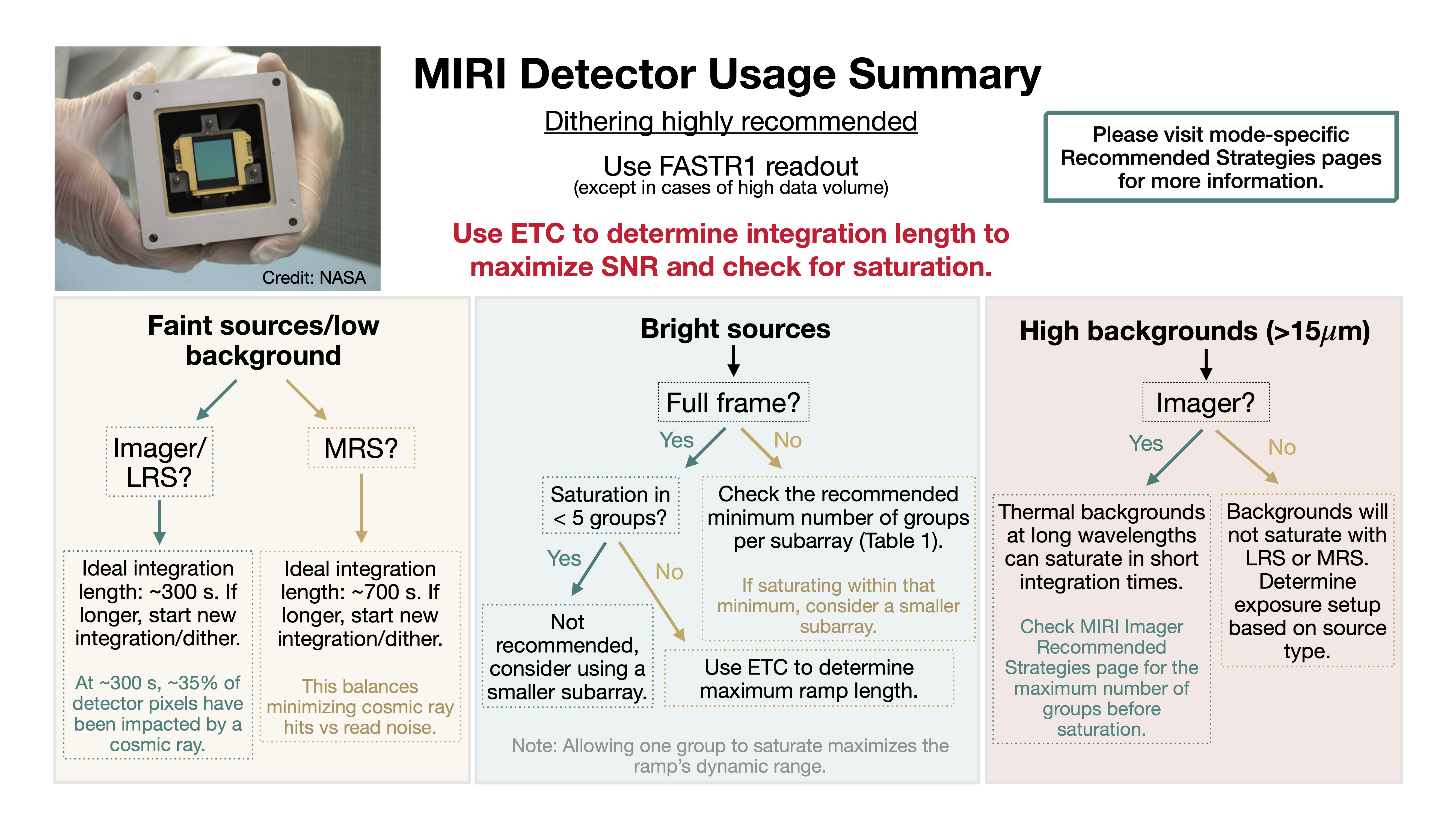
For MIRI the optimal combination of groups and integrations depends on the target brightness, the background and the desired signal-to-noise ratio. Users should use the ETC to evaluate the exposure time needed to achieve their scientific objectives and follow the guidelines below.
Click on the figure for a larger view.
For time-series observations, please see MIRI TSO Recommended Strategies.
What is the recommended ideal, minimum, and maximum length of an integration?
Words in bold are GUI menus/
panels or data software packages;
bold italics are buttons in GUI
tools or package parameters.
- The ideal number of groups is 100 FASTR1 groups (total time of ~300 s), which balances robust calibration against cosmic ray hits. However, the number of groups chosen will ultimately depend on the source brightness and background conditions:
- Bright sources/high background conditions will generally mean that saturation is reached in a short number of groups (5 to 10). Having one group saturating at the end of the integration will maximize the dynamic range. For very bright cases, imaging users should favor subarrays.
- Faint source observations will benefit from having longer integrations. In FASTR1 mode, 40 groups (about 100 s in FULL array, shorter when using subarray mode) is suggested as a starting point. Increase or decrease the integration to achieve your desired signal to noise. SLOWR1 or FASTGRPAVG8 are recommended primarily to limit data volume when MIRI imager is used simultaneously with MRS. See the MRS Recommended Strategies page for specific MRS guidance.
- Bright sources/high background conditions will generally mean that saturation is reached in a short number of groups (5 to 10). Having one group saturating at the end of the integration will maximize the dynamic range. For very bright cases, imaging users should favor subarrays.
- Minimum number of groups: The recommended minimum number of groups required to obtain a reasonable calibration are subarray- and readout pattern-dependent. Table 1 presents these recommendations for exposures with only 1 integration and exposures with more than 1 integration, as the detector effects are different in the first and subsequent integrations (see Gordon et al. 2025). These recommendations assume the FASTR1 readout pattern; recommendations are also made for the SLOWR1 and FASTGRPAVG8 readout patterns, which only apply for the FULL arrays. For very bright sources, observers are permitted to use fewer groups, but at this time there is no guideline for the noise and photometric accuracy we can expect. When using fewer than the recommended number of groups, and if photometric accuracy is important to your program, you should plan to observe a calibration star with exactly the same exposure parameters. If, instead of accuracy, repeatable precision is your primary need (e.g., transits), then this step may not be necessary.
Table 1. Recommended minimum number of groups for given subarrays and readout patterns
| Subarray or readout pattern | Recommended minimum groups for exposures with 1 integration | Recommended minimum groups for exposures with >1 integration |
|---|---|---|
| FULL | 4 | 5 |
| BRIGHTSKY | 4 | 7 |
| SUB256 | 5 | 8 |
| SUB128 | 10 | 10 |
| SUB128_IP† | 10 | 10 |
| SUB64 | 7 | 12 |
| SUB64_IP† | 7 | 12 |
| MASK1065 | 10 | 8 |
| MASK1140 | 9 | 9 |
| MASK1550 | 9 | 6 |
| MASKLYOT | 9 | 6 |
| SLITLESSPRISM | 8 | 10 |
| SLITLESSPRISM_IP† | 8 | 10 |
| SLITLESSPRISM_IPS† | 8 | 10 |
| SUBSLIT | N/A | N/A |
| MRS1/MRS2 FULL | 5 | 5 |
| SLOWR1 | 3 | 4 |
| FASTGRPAVG8† | 3 | 4 |
† Recommended minimum groups for subarrays added in Cycle 6 are notional until confirmed through analysis of on-sky data. For the time being, the recommendations match those of the comparable subarrays available in Cycle 5 and earlier, except for SUBSLIT, which has no prior equivalent. The same is true for the FASTGRPAVG8 readout pattern, which is given the same recommendation as SLOWR1 as a placeholder.
- Maximum recommended integration length: Based on in-flight experience, and considering the impact of the background, cosmic rays, cosmic ray showers, and other detector effects, 300 s is the maximum recommended integration length for imaging, coronagraphy and LRS observations. After 300 s about 35% of the MIRI detector pixels are affected by a cosmic ray, either as a direct or secondary impact of a cosmic ray, or a cosmic ray shower (see Figure 2, left). Integrations longer than 300 s may be desired in cases of very low background, such as those measured in the MIRI MRS where the data will be photon noise limited. For MRS, it is recommended that the maximum integration length be kept to ~700 s or less in order to limit cosmic ray effects. On-orbit measurements indicate that in a 1,000 s integration, most of the detector pixels are affected by cosmic rays (see Figure 2, right) and therefore that is the maximum recommended integration length. To understand cosmic ray treatment by the ETC visit the JWST ETC Cosmic Ray Implementation page.
Users are strongly encouraged to follow these general guidelines of integration length optimization. Please reach out to the JWST Help Desk with further questions.

Cosmic ray impact analysis on a single integration 1000 s (360 groups FASTR1) MIRI detector dark. Left: Number of pixels with one or more cosmic ray hits in a single 1,000 s integration (360 groups FASTR1) MIRI detector dark. Right: MIRI detector pixels flagged as impacted by a cosmic ray "jump". The color bar represents the total number of groups flagged either after the jump or due to multiple hits. The post-jump flagging is currently performed by default in the JWST calibration pipeline for all data but MRS, and the cosmic ray showers flagging is run by default for Imaging observations in filters F560W through F1500W.
How should I deal with saturation?
In many cases, the maximum integration length will be set by saturation of bright sources within the field, emission lines within a spectrum, or background emission. Because MIRI samples many points "up the ramp," saturating midway in the integration does not mean that data are lost; the pipeline will only fit the initial unsaturated data points. This can be an advantage since you can integrate longer to gain better signal to noise on fainter areas of the field or spectrum. However, saturation, as well as bright sources, can leave persistence artifacts in subsequent exposures (Dicken et al. 2024). Additionally, bright sources near saturation can cause a broadening effect on the PSF known as the "brighter-fatter" effect. High redundancy in the data (e.g., dithering) is strongly recommended to mitigate the effects of persistence.
When evaluating the impact of saturation as predicted by the ETC, users should keep in mind that the ETC is conservative, and does report saturation at about 80% of the detector full well. Further details can be found in the ETC Saturation Limits article.
For the special case of target acquisition, saturation should be avoided. Saturated pixels can cause the onboard centroiding algorithm to perform poorly, or fail, leading to the science observation being skipped.
Should I use multiple integrations?
The first integration within an exposure differs from the second and subsequent ones. This is because there are multiple detector resets between exposures (the system goes into a continuous reset while the telescope is dithering, filter wheels are moving, etc.), allowing some of the above-mentioned transient features to be cleared out of the first integration of the exposure. For multiple integration data the MIRI detectors use an additional reset (FASTR1, SLOWR1, and FASTGRPAVG8), which does allow for the majority of these transient effects to decay.
To decide whether to use multiple integrations, observers should consider various aspects: brightness of the source, detector performance, dithers, and overheads. These can all be captured in 2 broad cases:
- Bright sources/high backgrounds that saturate rapidly: in this case, multiple integrations allow building SNR on fainter regions while avoiding saturation on brighter targets. Saturation in the final group of the ramp does not generally affect the accuracy of calibration, i.e., is an acceptable strategy. Telescope maneuvers to the next dither position are more "costly" than starting a new integration.
- Fainter sources that can reach the "ideal exposure length" of 300 s (see above) will benefit from single integrations in all dither positions. It is best to select integration lengths which are as long as your observations allow (i.e., a few long integrations are better than many shorter ones).
Choosing the readout mode: FASTR1 vs. SLOWR1 or FASTGRPAVG8
See also: MIRI Detector Readout Overview
FASTR1 is the recommended readout mode for all MIRI observations executed as prime. SLOWR1 mode is useful for parallel observations and in some MRS programs, where it can be essential to limit the data volume. However, SLOWR1 will be deprecated in a future cycle and users are encouraged to begin using FASTGRPAVG8 in Cycle 6.
The MIRI detectors can be operated using 3 different readout modes for science exposures: FASTR1, SLOWR1, and FASTGRPAVG8. For Target Acquisition, additional FASTRGRPAVG combinations are available to maximize signal-to-noise. The main differences between these modes are:
- FASTR1 mode reads out the detector every 2.775 s in full array mode, vs. 23.889 s for SLOWR1 and 22.20 s for FASTGRPAVG8. The FASTR1 mode offers finer time sampling that allows better characterization of detector effects and more samples for cosmic ray correction. Compared to SLOWR1 and FASTGRPAVG8, in the FASTR1 mode there is approximately a factor of 9 and 8 less time lost in case of a cosmic ray hit, respectively.
- SLOWR1 mode provides about 9 times less data volume. SLOWR1 is only recommended to mitigate data volume concerns encountered when using FASTR1.
- FASTGRPAVG8 reduces data volume by a factor of 8 by co-adding 8 consecutive frames into a single group. This readout mode can be used in any situation where SLOWR1 is recommended.
Programs should not have both readout patterns FASTR1 and SLOWR1 set in the same observation, for the same detector. Changing between these patterns adds noise as there is a thermal difference between the two readout patterns, and the detectors need to settle after a switch. Having different readout modes for different detectors does not have the same issue, i.e., MRS can be set to SLOWR1, while simultaneous imaging is set to FASTR1. Note that there is no settling time required between FASTR1 and FASTGRPAVG8 because the latter is simply an onboard average of the former, so these two modes can be safely specified in the same observation.
Background observations recommendations
See also: JWST Background Model, JWST Background-Limited Observations
Does my program need background observations?
Please read the following pages for MIRI mode-specific guidance on backgrounds:
MRS Dedicated Sky Observations
MIRI Imaging Recommended Strategies
MIRI LRS Recommended Strategies
MIRI Coronagraphic Recommended Strategies
MIRI WFSS Recommended Strategies
Observers should carefully consider the impact the extra emission of the JWST background (modeled by the JWST ETC Backgrounds) will have on their data. Please refer to JWST Background-Limited Observations for guidelines on how to use the Background Limited special requirement in APT.
How often do I need to get a background?
The JWST mission defines visits as individual schedulable units, used to build up the observation timeline. Visits that are not linked by special requirements can be planned at different times of the observing cycle and background variations are expected. Observers should plan on taking background data for every observing period (i.e., non-linked visit) in their programs.
The JWST Background Variability provides information on the spatial and temporal variability of the background.
Observing programs that need low backgrounds can request visits to be scheduled when the background is predicted to be relatively low. Observing programs that require high accuracy relative calibrations in the results (better than 1%) and use extended targets may consider taking background data before and after the science exposures. Users are encouraged to use the JWST Backgrounds Tool to better understand the impact of the background in their observations, its intensity, and components as a function of time.
Target acquisition
An overview of the MIRI target acquisition process is given elsewhere in the documentation and discussed in the mode-dedicated target acquisition articles (MIRI Imaging Target Acquisition, MIRI MRS Target Acquisition, MIRI LRS Slit Target Acquisition, and MIRI LRS Slit Target Acquisition). These articles also include guidelines on when TA is needed for each MIRI mode.
TA targets
See also: MIRI Target Acquisition
When TA is needed (see JWST Pointing Performance) the science target is typically used for TA. However, the procedure can also be carried out with a nearby bright star, which should be within the APT visit splitting distance of the science target. The splitting distance typically ranges between 30" and 80", depending on the Galactic latitude of the target, and is defined as the total distance between the TA and science exposures which is the combination of:
- The distance between the TA target and science target.
- The distance between the TA aperture and the science aperture.
If the TA target is not within this visit splitting distance, the observation may not be schedulable by the APT Visit Planner. Users are encouraged to check whether their program can be scheduled when using off-source TA targets. The accuracy of this TA is limited by the precision of the difference between the offset and science targets.
If feasible, using an offset TA target should be considered in the following scenarios:
- The science target is spatially resolved, resulting in a higher uncertainty on the centroid location (see section below).
- The science target's spectral energy distribution is not well known in the MIRI TA filters, leading to an uncertain estimation of the exposure time and SNR.
- The science target requires a long (~100 s or longer) integration to reach an SNR of 50.
Understanding the TA onboard procedure
The aim of this section is to give details on the onboard TA data process, so users understand the several aspects that might impact its accuracy/outcome. The onboard centroid algorithm for MIRI works as follows:
- The onboard algorithm uses the first, middle and one-before-last frame to generate two 2-frame difference images. The final image used for TA is then constructed by taking the minimum value of these 2 difference images on a pixel by pixel basis.
- This raw image is pre-treated (background subtracted and flat fielded).
- It then finds the brightest 5 × 5 pixel region of the detector region of interest (ROI, see Table 2). The checkbox size (5 × 5) has been defined to encompass the imager PSF.
- After that, it performs a fine location by calculating the center of mass in the previously located brightest area.
The accuracy of this procedure depends on several aspects:
- The TA target should be a point source.
- The recommended minimum SNR of the TA image is 50.
- The TA source should be the brightest source in the ROI. If there is a source of comparable brightness, or brighter, than the intended target, there is a high risk of the algorithm returning the interloper's centroid. If there is a source with the same brightness the algorithm will perform TA in the first one encountered following the direction in which the detector is read out.
- Users should be aware that regions with bright diffuse emission may also result in false identification of the TA target. To reduce the possibility of this happening, the checkbox area is a very small one.
Table 2. Sizes of detector regions of interest used to perform target acquisition.
| TA region of interest (ROI) | Size |
|---|---|
| MRS (TA performed in imager detector) | 48 × 48 pixel2 |
| LRS (slit and slitless) | 48 × 48 pixel2 |
| Coronagraphs | 48 × 48 pixel2 (16 × 16 pixel2 secondary TA) |
Note that the MIRI detector plate scale is 0.11 arcsec/pix.
Additional information is available in these articles:
MIRI Imaging Target Acquisition
MRS MIRI MRS Target Acquisition
MIRI LRS Slit Target Acquisition
MIRI LRS Slit Target Acquisition

In this example of a rich field, if the observer selects the central star as a TA target, the centroid algorithm will not be performed there but in the brightest pixel of the field (top right). After the TA is performed on the wrong target, data will not be taken at the coordinates of the science target specified in the proposal. Observers are encouraged to carefully select the TA target so that there are no brighter neighbors.
Target acquisition readout mode: FAST and fast group averaging
MIRI target acquisition can be performed using 6 different readout modes: FAST (FASTR1 is not used for TA),and 5 different flavors of fast group averaging (see MIRI Target Acquisition). A maximum of 10 FULL-frame groups can be held in memory for the TA algorithm. To allow for longer TA exposures, FASTRGRPAVG readout modes are available with group averaging of 4, 8, 16, 32, and 64 groups. Fast group averaging is offered for MIRI TA only, with the lone exception being FASTGRPAVG8, which is available for science observations. The ETC will give warnings when the SNR achieved is not sufficient to successfully finish the TA procedure (see more details in JWST ETC MIRI Target Acquisition).
References
Dicken, D. et al. 2024, A&A, 689, A5
JWST MIRI Flight Performance: Imaging
Gordon, K. D. 2025, JWST-STScI-009097, SM-12
MIRI Reset Switch Charge Decay (RSCD): Quantitative Measurement of Number of Groups Affected
Krick J. E. et al., 2012, ApJ, 754, 53
A Spitzer/IRAC Measure of the Zodiacal Light
Lightsey, P.A., 2016, SPIE, 9904, 99040A
Stray light field dependence for the James Webb Space Telescope
Morrison, J. E. et al. 2023, PASP, 135, 075004
JWST MIRI Flight Performance: Detector Effects and Data Reduction Algorithms
Ressler et al. 2015, PASP, 127, 675R
The Mid-Infrared Instrument for the James Webb Space Telescope, VIII: The MIRI Focal Plane System
Rieke et al. 2015, PASP, 127, 665R
The Mid-Infrared Instrument for the James Webb Space Telescope, VII: The MIRI Detectors