Sample code
# The following section is only needed if the PYSYN_CDBS environment variable is not already set.
# The PYSYN_CDBS environment variable should point to the path of the CDBS data files
import os
location_of_cdbs = "/path/to/cdbs/files"
os.environ['PYSYN_CDBS'] = location_of_cdbs
# End section
# The following section is only needed if the pandeia_refdata environment variable is not already set
# The pandeia_refdata environment variable should point to the path of the pandeia reference data
import os
location_of_pandeia_refdata = "/path/to/pandeia/refdata"
os.environ['pandeia_refdata'] = location_of_pandeia_refdata
location_of_psf_dir = "/path/to/pandeia/psfs"
os.environ["PSF_DIR"] = location_of_psf_dir
# End section
import numpy as np
from matplotlib import pyplot as plt
from pandeia.engine.calc_utils import build_default_calc
from pandeia.engine.perform_calculation import perform_calculation
# The following are parameters which can easily be changed
telescope = 'jwst'
instrument = 'miri'
mode = 'coronagraphy'
# Flux Range parameter
flux_range = np.linspace(0.1, 5e5, 15) #mJy
# Create lists to store the output data
tot_none, tot_soft, tot_hard = [], [], []
for flux in flux_range:
configuration_dictionary = build_default_calc(telescope, instrument, mode)
configuration_dictionary['scene'][0]['spectrum']['normalization']['norm_flux'] = flux
report_dictionary = perform_calculation(configuration_dictionary)
saturation = report_dictionary['2d']['saturation']
unsaturated = len(saturation[saturation==0.])
soft_saturated = len(saturation[saturation==1.])
hard_saturated = len(saturation[saturation==2.])
tot_none.append(unsaturated)
tot_soft.append(soft_saturated)
tot_hard.append(hard_saturated)
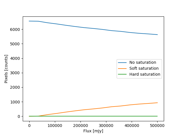
plt.plot(flux_range,tot_none, label='No saturation')
plt.plot(flux_range,tot_soft, label='Soft saturation')
plt.plot(flux_range,tot_hard, label='Hard saturation')
plt.xlabel('Flux [mJy]')
plt.ylabel('Pixels [counts]')
plt.legend()
plt.show()
The result of the above is shown in Figure 1.
Determining the number of groups needed to reach a signal to noise of 40 in a NIRCam SW observation
# The following section is only needed if the PYSYN_CDBS environment variable is not already set.
# The PYSYN_CDBS environment variable should point to the path of the CDBS data files
import os
location_of_cdbs = "/path/to/cdbs/files"
os.environ['PYSYN_CDBS'] = location_of_cdbs
# End section
# The following section is only needed if the pandeia_refdata environment variable is not already set
# The pandeia_refdata environment variable should point to the path of the pandeia reference data
import os
location_of_pandeia_refdata = "/path/to/pandeia/refdata"
os.environ['pandeia_refdata'] = location_of_pandeia_refdata
location_of_psf_dir = "/path/to/pandeia/psfs"
os.environ["PSF_DIR"] = location_of_psf_dir
# End section
from matplotlib import pyplot as plt
from pandeia.engine.calc_utils import build_default_calc
from pandeia.engine.perform_calculation import perform_calculation
from scipy import interpolate
# The following are parameters which can easily be changed
telescope = 'jwst'
instrument = 'nircam'
mode = 'sw_imaging'
filter = 'f115w'
# Source parameters
offsets = {'x': 0., 'y': 0.}
geometry = 'point'
name = 'G2V Star'
sed = 'phoenix'
key = 'g2v'
bandpass = 'sdss,r'
magnitude = 26.
scene_dictionary = {}
scene_dictionary['position'] = {'position_parameters': ['x_offset', 'y_offset']}
scene_dictionary['position']['x_offset'] = offsets['x']
scene_dictionary['position']['y_offset'] = offsets['y']
scene_dictionary['shape'] = {'geometry': 'point'}
scene_dictionary['spectrum'] = {'name': name, 'spectrum_parameters': ['sed', 'normalization']}
scene_dictionary['spectrum']['sed'] = {'sed_type': sed, 'key': key}
scene_dictionary['spectrum']['normalization'] = {'type': 'photsys', 'norm_fluxunit': 'abmag'}
scene_dictionary['spectrum']['normalization']['bandpass'] = bandpass
scene_dictionary['spectrum']['normalization']['norm_flux'] = magnitude
scene_dictionary['spectrum']['lines'] = []
scene_dictionary['spectrum']['extinction'] = {'bandpass': 'j', 'law': 'mw_rv_31', 'unit': 'mag', 'value': 0}
# Number of observation Groups for search
min_groups = 0
max_groups = 28
# Target SNR
target_sn = 40.
# Create lists to hold the results
sns, exptimes = [], []
while min_groups <= max_groups:
configuration_dictionary = build_default_calc(telescope, instrument, mode)
configuration_dictionary['scene'][0] = scene_dictionary
configuration_dictionary['configuration']['instrument']['filter'] = filter
current_groups = (min_groups+max_groups)//2
configuration_dictionary['configuration']['detector']['ngroup'] = current_groups
report_dictionary = perform_calculation(configuration_dictionary)
current_sn = report_dictionary['scalar']['sn']
sns.append(current_sn)
exptimes.append(report_dictionary['scalar']['total_exposure_time'])
if current_sn <= target_sn:
min_groups = current_groups + 1
else:
max_groups = current_groups - 1
interpolator = interpolate.interp1d(sns,exptimes)
exptime_target = interpolator(target_sn)
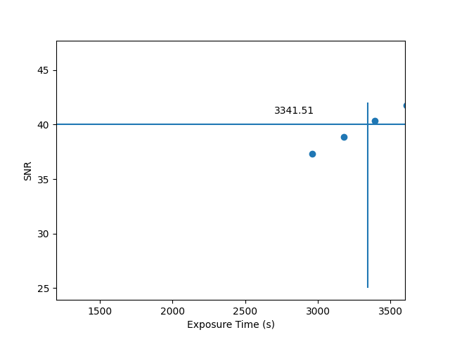
print("For SNR=40: {:.2f}s".format(exptime_target))
print("Groups: {} Exptime: {:.2f}s SNR: {:.2f}".format(min_groups,exptimes[-1], sns[-1]))
plt.scatter(exptimes,sns)
plt.hlines(40,1200,3600)
plt.vlines(exptime_target,25,42)
plt.xlabel('Exposure Time (s)')
plt.ylabel('SNR')
plt.text(2700,41,"{:.2f}".format(exptime_target))
plt.xlim((1200,3600))
plt.show()
The result of the above is shown in Figure 2.
Determining date with lowest background flux at given coordinates
from __future__ import division

# The following section is only needed if the PYSYN_CDBS environment variable is not already set.
# The PYSYN_CDBS environment variable should point to the path of the CDBS data files
import os
location_of_cdbs = "/path/to/cdbs/files"
os.environ['PYSYN_CDBS'] = location_of_cdbs
# End section

# The following section is only needed if the pandeia_refdata environment variable is not already set
# The pandeia_refdata environment variable should point to the path of the pandeia reference data
import os
location_of_pandeia_refdata = "/path/to/pandeia/refdata"
os.environ['pandeia_refdata'] = location_of_pandeia_refdata
location_of_psf_dir = "/path/to/pandeia/psfs"
os.environ["PSF_DIR"] = location_of_psf_dir
# End section
import numpy as np
from matplotlib import pyplot as plt
from pandeia.engine.calc_utils import build_default_calc
from pandeia.engine.perform_calculation import perform_calculation

from jwst_backgrounds import jbt

# Background Flux Parameters
ra = 129.4
dec = 41.1
background_primary_wavelength = 4.0 # in microns, doesn't actually matter as we want the full spectrum.


# General Observation Parameters
telescope = 'jwst'
instrument = 'nircam'
mode = 'sw_imaging'
filter = 'f090w'

# Source parameters
offsets = {'x': 0., 'y': 0.}
geometry = 'point'
name = 'G2V Star'
sed = 'phoenix'
key = 'g2v'
bandpass = 'sdss,r'
magnitude = 22.

bg = jbt.background(ra, dec, background_primary_wavelength)
wave_array = bg.bkg_data['wave_array']
observability_calendar = bg.bkg_data['calendar']

scene_dictionary = {}
scene_dictionary['position'] = {'position_parameters': ['x_offset', 'y_offset']}
scene_dictionary['position']['x_offset'] = offsets['x']
scene_dictionary['position']['y_offset'] = offsets['y']
scene_dictionary['shape'] = {'geometry': 'point'}
scene_dictionary['spectrum'] = {'name': name, 'spectrum_parameters': ['sed', 'normalization']}
scene_dictionary['spectrum']['sed'] = {'sed_type': sed, 'key': key}
scene_dictionary['spectrum']['normalization'] = {'type': 'photsys', 'norm_fluxunit': 'abmag'}
scene_dictionary['spectrum']['normalization']['bandpass'] = bandpass
scene_dictionary['spectrum']['normalization']['norm_flux'] = magnitude
scene_dictionary['spectrum']['lines'] = []
scene_dictionary['spectrum']['extinction'] = {'bandpass': 'j', 'law': 'mw_rv_31', 'unit': 'mag', 'value': 0}

# Create lists to hold the results
dates, fluxes = [], []


for i, day in enumerate(observability_calendar):
    configuration_dictionary = build_default_calc(telescope, instrument, mode)
    configuration_dictionary['scene'][0] = scene_dictionary
    configuration_dictionary['configuration']['instrument']['filter'] = filter
    flux_array = bg.bkg_data['total_bg'][i]
    configuration_dictionary['background'] = [wave_array, flux_array]
    report_object = perform_calculation(configuration_dictionary, dict_report=False)
    background_rate = np.median(report_object.bg_pix) # median per-pixel background count rate
    print("Day {} has flux {}".format(day, background_rate))
    dates.append(day)
    fluxes.append(background_rate)

plt.scatter(dates,fluxes)
plt.xlabel("Day of Observation")
plt.ylabel("Background Count Rate (cnt/s)")

plt.show()
Figure 3 shows the background count rate on each day over the next year that the target is observable. As can be seen, observations near the start and end of the year offer the lowest background rate, although the overall difference is relatively small.