MIRI MRS Known Issues
Known issues specific to MIRI MRS data processing in the JWST Science Calibration Pipeline are described in this article. This is not intended as a how-to guide or as full documentation of individual pipeline steps, but rather to give a scientist-level overview of issues that users should be aware of for their science.
On this page
Specific artifacts are described in the Artifacts section below. Guidance on using the pipeline data products is provided in the Pipeline Notes section along with a summary of some common issues and workarounds in the summary section.
Please also refer to MIRI MRS Calibration Status for an overview of the current astrometric, wavelength, and flux calibration of MIRI MRS data products.
Artifacts
Bad pixels
Over time the number of bad and/or warm pixels on the MIRI MRS detectors has been increasing, resulting in salt & pepper noise in the 2-D calibrated detector images. While many of these are caught by the outlier detection step in the calwebb_spec3 pipeline prior to combination of the data into final dither-combined 3-D data cubes, some bright pixels nonetheless make it through into the cubes. These can be particularly noticeable in mosaic observations, as the same artifact will show up in multiple regular locations throughout the composite data cube (see Figure 1).
In January 2024 (CRDS context 1185) the MRS bad pixel masks were updated with new bad pixel masks for every 6 months of the mission, with 3 different flagging thresholds for shallow, medium, and deep observations. Shallow observations (defined as FASTR1 data with fewer than 50 groups) have the most permissive mask, flagging only the brightest warm pixels that would be visible above the detector readout noise. Medium observations (defined as FASTR1 data with 50 or more groups) flag more pixels, corresponding to the lower effective detector noise. Deep observations (defined as any SLOWR1 data) use the most aggressive masking, flagging approximately 4 times as many pixels as the shallow mask. Regular updates will continue to be delivered throughout the mission.
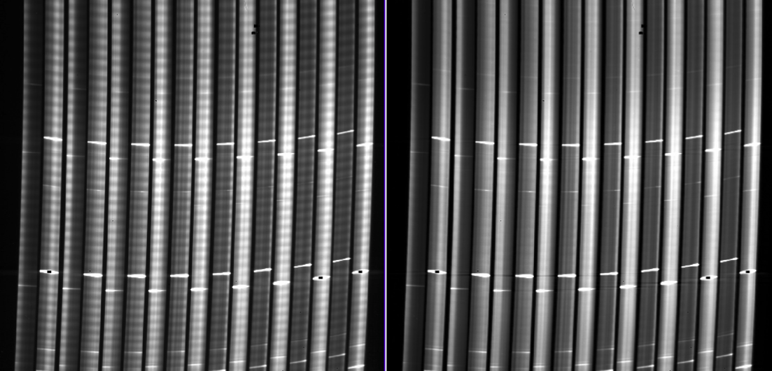
Figure 2 illustrates an example calibrated Ch3/Ch4 detector image before and after this update, noting the substantial improvement in data quality provided by the pixel replacement routine interpolating across newly identified bad pixels.
For any remaining artifacts, it can be helpful to use dedicated background observations taken with the science data to generate and apply a custom bad pixel mask.

Click on the figure for a larger view.
Images of an MRS mosaic data cube showing typical bad pixel artifacts (circled in red); since these correspond to a fixed location on the detector they show up at regular locations in the final cube. In this case, the pair of nearby artifacts is produced by a 2-pt dither, which is repeated 4 times as this is a 2 × 2 mosaic. Artifacts can be either positive or negative. Bright green pixels represent NaN-valued regions outside the IFU footprint.

Click on the figure for a larger view.
Section of a calibrated long wavelength detector image (cal.fits) for an MRS 33-group SLOWR1 dedicated background observation processed with two different sets of bad pixel mask reference files. The image on the right shows significantly better bad pixel suppression, resulting in many fewer outliers that would otherwise need to be identified during the outlier_detection routine. NaN-valued pixels are shown as black in this representation.
Cosmic ray showers
See also: Shower and Snowball Artifacts
Cosmic ray shower correction is off by default for MIRI MRS in pipeline build 10.1 and earlier due to some known failure cases when used on very bright targets (for which shower correction is typically unnecessary anyway). Users working with deep observations of faint targets may benefit the most from enabling shower corrections in offline reprocessing. Note that there is a known bug in pipeline versions 1.13.4 and earlier that the shower correction code does not successfully run on data using the SLOWR1 readout pattern. This bug has been corrected in more recent versions of the pipeline.
Cruciform artifact
Please refer to MIRI Known Issues.
Fringing
As discussed in depth by Argyriou et al. 2020, like most IR spectrometers, the MRS experiences strong spectral fringing of order 10%–30% of the incident spectral baseline at all wavelengths. These large-amplitude sensitivity modulations are caused by constructive and destructive interference produced by multiple internal reflections within different layers of the MIRI detectors. On the LONG wavelength detector, there is an additional low amplitude high frequency modulation attributed to fringing within the dichroic optical elements. While the fringe frequencies are well known, amplitudes can vary due to beating between the different fringe components and additionally are sensitive to the detailed location and intensity of objects within a given astronomical scene. Fringing thus cannot be corrected in its entirety for an arbitrary astronomical scene without forward modeling.
Multiple pipeline steps exist, however, to mitigate the impact of this fringing on science spectra and these steps generally suffice to reduce the fringe signal to below a few percent of the target flux.
The first step, applied by default in the JWST pipeline, is to divide the uncalibrated "rate" image by a static fringe flat constructed from observations of a bright source that fills the entire MRS field of view. This step generally does a good job of removing the strongest fringes from an astronomical scene, particularly for nearly-uniform extended sources (see Figure 3). Since the fringe signal is different for point sources however (and varies as a function of the location of a point source within the FOV) the static fringe flat cannot fully correct such objects and the default high level data products will therefore still show appreciable fringes.
The pipeline also includes two optional residual fringe correction steps whose purpose is to find and remove signals whose periodicity is consistent with known fringe frequencies (set by the optical thickness of the detectors and dichroics) using a Lomb-Scargle periodogram (see details given by Kavanagh et al. 2023). The number of fringe components to be removed is governed by a Bayesian evidence calculation. The first of these residual fringe correction steps is a 2-D correction that can be applied to the flux-calibrated detector data in the calwebb_spec2 pipeline by enabling the residual_fringe step. The second of these residual fringe correction steps is a 1-D correction (in the jwst pipeline version 1.11.0 and later) that can be applied to one-dimensional spectra extracted from MRS data cubes by setting the optional parameter extract_1d.ifu_rfcorr = True. Empirically, the 1-D correction step has been found to both work better than the 2-D correction step and is much faster for the pipeline as well.
This 1-D residual fringe correction can also be applied to user-extracted spectra as well. Given a numpy array of wavelengths wave and fluxes flux, the routine can be called in a standalone fashion for spectra from Channel 4 as
from jwst.residual_fringe.utils import fit_residual_fringes_1d as rf1d
flux_cor = rf1d(flux, wave, channel=4)
and analogously for spectra from any other channel.
As illustrated in Figure 4, the residual fringe correction step can work well to remove periodic fringes from the spectra of bright point sources. However, its utility is nonetheless limited in a few key ways. First, since the fringe frequencies change with wavelength, the 1-D residual fringe correction performs best when applied to spectra extracted from a single one of the 12 MRS bands at a time and does not generally work when applied to full 5–28 µm spectra across the entire MRS wavelength range. Second, the step relies upon being able to measure periodic amplitude modulations in the data. If a given spectrum is too faint, or if it contains too much astrophysical structure to reliably isolate the fringe signal, the residual fringe routine will not perform well. Finally, if the science target contains genuine astrophysical structure with frequencies similar to the known fringe frequencies (e.g., as is the case for some icy debris disks) then the residual fringe routine can remove this astrophysical signal from the data.
Work is underway during Cycle 2 to explore additional corrections for fringing (e.g., using finely sampled templates of point sources stepped across sub-pixel samples), and further updates will be provided as they become available.
Click on the figure for a larger view.
Left panel: Section of a calibrated detector image showing observations of a bright planetary nebula filling multiple IFU slices. White lines are nebular emission, while alternating bright and dark features are produced by detector fringes modulating the observed amplitude of the continuum emission. Right panel: As left panel, but after application of the static fringe flat. Note that the alternating bright and dark fringe features have been almost entirely removed.

Click on the figure for a larger view.
Channel 2B spectra extracted from observations of the bright O star 10 Lac (blue line). The periodic amplitude modulations in the continuum are due to residual fringes not well corrected by the static fringe flat. Application of the 1-D residual fringe routine almost entirely removes these residual fringes from the spectrum (orange line).
Resampling noise
As discussed in MIRI MRS PSF and Dithering, the MRS is spatially undersampled by a factor of about 2 compared to the Nyquist sampling necessary to fully reconstruct the PSF delivered by the JWST optics. As a result, when the cube building software resamples the native detector pixel data into a regular cube grid there are artifacts produced by the resampling for unresolved point sources. This issue is explored in detail by Law et al. 2023. In brief, the size of the artifact is related to the pixel phase of the dispersed trace centroid; since the trace centroid curves across the detector these artifacts appear as sinusoidal variations in the reconstructed intensity whose frequency varies with wavelength according to the rate at which the trace crosses pixel boundaries.
Figure 5 shows the theoretically expected resampling artifacts for MRS channel 1A based on a model of the JWST PSF and MIRI MRS detector sampling; these are similar to actual artifacts observed in the spectra of bright point sources with data obtained during Cycle 1. In both simulated and observed cases, the resampling noise is significantly reduced by obtaining data using a 4-point dither pattern designed to properly sample the JWST PSF. Even for a 4-point dither pattern however, few-percent artifacts remain if attempting to plot the spectra of individual spaxels from the data cubes. Essentially, doing so is akin to a 2-D case of comparing the brightness of multiple stars throughout an undersampled image by looking only at the brightest central pixel values. As in the 2-D case, extracting photometric information from an aperture comparable to the PSF FWHM in size reduces the amplitude of the artifacts to well below 1%, ensuring flux conservation in an integrated sense.
In large part, such resampling artifacts are unavoidable as they result directly from the undersampling of the MRS optics. However, work is currently ongoing to study whether some science cases can admit corrections that enforce smoothness on sub-PSF scales, either by forward modeling the detector data or applying empirical post-facto corrections based on the known phase crossing frequency of the dispersed point source traces. Further information will be provided here as it becomes available.

Click on the figure for a larger view.
Left panels: Numerical model of expected artifacts in channel 1A for undithered, 2-pt dither, and 4-pt dithered data for spectra extracted using apertures of various sizes (ranging from single-spaxel spectra to apertures with radii twice the PSF FWHM). Right panels: Observed resampling noise in observations of G3V standard star 16 CygB. The overall tilt in the 16 CygB spectrum is due to the intrinsic spectral shape of the star. (Figure credit: Law et al. 2023)
Spectral leak
The MIRI MRS filters are designed to keep out-of-band light from interfering with the desired first order wavelengths dispersed in a given band. However, around 12.2 µm (channel 3A) a few-percent spectral leak admits second-order light from 6.1 µm (channel 1B) into the bandpass. As a result, very blue sources with a large amount of flux at 6.1 µm can show a bump of additional emission in their 12.2 µm spectrum.
As of JWST pipeline version 1.13.0 and CRDS reference file version jwst_1150.pmap, the spectral leak pipeline step corrects for this leak for 1-D spectra extracted from point source targets by convolving the 6 µm spectrum with the known leak response function and subtracting the result from the 12 µm spectrum. The results of this correction for both a very-blue (G-type star HD 2811) and a very-red source (asteroid 515 Athalia) are illustrated in Figure 6.
Note that in early versions of the photometric calibration reference files (prior to jwst_1094.pmap) the spectral leak was not corrected when deriving the 12 µm photometric responsivity curve, effectively baking the leak from an A-type star into the calibration. As a result, with these early reference files the spectral leak tended to manifest as an artificial dip in the spectra of red sources rather than excess flux in the spectra of blue sources.
Note also that no such spectral leak correction is available for the 3-D IFU data cubes or for extracted spectra of extended sources; since the 12 µm field of view extends beyond the 6 µm field of view, the shorter wavelength data cannot be used to correct the 12 µm data throughout the field of view.

Click on the figure for a larger view.
Extracted 1-D spectra of a blue source (A-type star HD 2811) and a red source (Asteroid 515 Athalia) with and without correction for the 12.2 µm spectral leak. Spectral leak correction makes no discernible difference to the red spectrum as there is little light at 6 µm to contaminate the 12 µm region. Figure credit: Law et al. (in prep)
Time-dependent count rate loss
See MIRI MRS Calibration Status
Pipeline notes
The MIRI MRS pipeline is complex, and there are multiple points that users should keep in mind for individual stages that can affect the quality of the final data products.
WCS accuracy
As discussed in MIRI MRS Calibration Status, the MRS data products have a typical global WCS uncertainty of about 0.3" (1-σ radial) due to the guide star catalog and spacecraft roll uncertainty. This global uncertainty applies even in the case for which target acquisition was performed and the science target correctly placed at the intended location within the instrument, and can in rare cases be as large as 1.5". This is a systematic offset that tends to be a single linear shift that is the same for all exposures within a given observation, and as such can be corrected using MIRI simultaneous imaging. If sources with known (e.g., Gaia) positions fall within the MIRI imaging FOV these can be used to derive the necessary RA/DEC shift of the MIRI (imaging + MRS) data; these values then need to be added to the RA_REF, DEC_REF keywords of the IFU "rate.fits" file header, and the calwebb_spec2/calwebb_spec3 pipeline rerun to incorporate that information. A notebook demonstrating this procedure will be made available during Cycle 2.
At a lower level, the non-repeatability of the MRS grating wheel imposes an uncertainty floor of a few hundredths of an arcsecond relative to the MIRI imager. This results in a small offset ~ 1/10 of the PSF FWHM between individual MRS bands which can be noticeable when plotting spectra of individual spaxels near the centers of point sources.
See the guidance below for how to mitigate the impact of these effects on spectral extraction.
Background subtraction
The MIRI MRS sees a significant component of background light at long wavelengths, both from reflected zodiacal light and from JWST thermal emission (particularly in channel 4). As such, it is important to subtract this background signal in order to measure the astrophysical signal of interest. There are presently 3 locations at which this can happen for MIRI MRS in the pipeline:
- Background subtraction (calwebb_spec2): This performs pixel-by-pixel background subtraction in which one exposure can be directly subtracted from another, removing a background signal but introducing noise from both the science and background exposures into the final image (especially if both suffer from large cosmic ray showers). This approach is not used by the pipeline unless manually specified to do so, and analysis of Cycle 1 data shows that it is not beneficial in most cases.
- Master background subtraction (calwebb_spec3): This subtracts the background signal from science data using a one-dimensional master background spectrum. This master background spectrum is typically created by combining all 1-D spectra from dedicated background observations processed by the calwebb_spec2 pipeline, and broadcast to the entire 2-D detector array by interpolating to the wavelengths of each detector pixel. This broadcast array is then subtracted from the individual 2-D science frames with little to no degradation of the SNR (since it uses a 1-D spectral model produced from the sigma-clipped combination of many detector pixels rather than the values of those pixels themselves). Alternatively, users can provide a custom 1-D background spectrum, which must be specific in surface brightness units of MJy/sr. A few key notes:
- This step does not run by default unless there is a dedicated background observation properly linked to the science observations. Science data cubes for programs that did not include dedicated backgrounds will not be background-subtracted unless users create and provide a custom 1-D background spectrum to the master background routine.
- If data are designated as linked background observations, then extract_1d will use the entire field of view as the extraction region. The master_background step recognizes the type of background exposure and uses the appropriate "x1d" data product to produce the master background.
- At present, the master background spectrum can have arbitrary spectral structure. Possible future revisions to this routine are under consideration that would enforce a background model that varies smoothly as a function of wavelength, helping to reduce noisy artifacts from cosmic ray showers that can remain even after sigma-clipping throughout the field of view.
- Annular background subtraction during spectral extraction
- (calwebb_spec2): If processing any target indicated as a point source, the extract_1d step will compute a background spectrum using a sigma-clipped algorithm in an annulus surrounding the location of the source. By default, this background spectrum will be subtracted from the 1-D science spectrum extracted from the circular aperture centered on the source (accounting for the effective area of that aperture). Both the background annulus and circular aperture increase in size with wavelength.
- (calwebb_spec3): As in calwebb_spec2, the process of spectral extraction from a 3-D data cube for point sources by default applies a background subtraction from an annular region surrounding a point source. Even in cases for which master background subtraction was already done, the annular background subtraction should be performed since the aperture correction factors applied to the data are derived assuming that the fraction of the PSF contained within the background annulus has been subtracted from the data.
Outlier detection
Despite the jump step in the calwebb_detector1 pipeline flagging jumps due to cosmic rays in the ramps of individual pixels, outliers can nonetheless persist into the calibrated 2-D data products and cause unphysical spikes in the extracted 1-D spectra. The majority of these outliers are due to warm pixels that are not flagged in the bad pixel mask.
In standard imaging modes, the approach to outlier detection is to create a version of the final scene from each input frame, median these together to get a "clean image," and blot this back to the detector frame of individual exposures to identify any outliers. Since the MRS is severely undersampled (see MIRI MRS PSF and Dithering) this resampling both forward and backward from individual exposures results in significant artifacts around unresolved point sources. These artifacts can confuse such projection-based outlier detection algorithms (a version of which was implemented in commissioning and early Cycle 1), resulting in both poor rejection of outliers and occasional rejection of some spectral segments of genuine point sources.
Since jwst pipeline version 1.11.0 and greater, an algorithm for outlier detection has been implemented that uses a more classical approach from CCD image processing to identify sharp features on the detector that are inconsistent with the known detector PSF. This approach does substantially better at flagging real outliers while not flagging science signal in the many possible kinds of JWST targets, and runs many times faster than the original algorithm. While an improvement on the original routine, outlier detection is still imperfect and some outliers can remain in the data cubes and extracted spectra for some science programs. As additional improvements are tested the corresponding algorithms will be updated as necessary.
Cube building
The cube_build step combines the individual 2-D frames of dispersed IFU data to create a regularized 3-D spectral cube. By default, cube building uses a 3-D variant of the classical drizzle algorithm to apportion the flux to individual cube voxels based on the relative volumetric overlap between the output voxels and the input detector pixel footprint, although an alternative method using a flux-conserving version of Shepard's method with an exponential weighting kernel (EMSM) is also available. Both algorithms are described by Law et al. 2023 and have similar performance although the 3-D drizzle approach provides data cubes with a slightly sharper PSF since the exponential weighting inherent in the EMSM approach effectively smooths the data cubes by a small kernel function. (This smoothing can, however, also serve to partially mitigate the impacts of resampling noise). The cube building algorithm can be selected using the weighting argument to cube_build:
calwebb_spec3.cube_build.weighting = 'drizzle' or 'emsm'
The FOV, slice width, number of slices, spectral resolution, and plate scales are different for each channel. The cube_build step will use the "cubepar" reference file (e.g., jwst_miri_cubepar_0012.fits) to determine the proper defaults for the spaxel scale and wavelength sampling of a given IFU data cube (see discussion by Law et al. 2023). If building cubes from a single MRS band (e.g., 1A) or channel (e.g., 2A + 2B + 2C) the resulting IFU cube will have a linearly-spaced step in the wavelength dimension. Cube building can also combine together data from multiple different channels (e.g., Ch1 + Ch2), in which case the IFU cube will have a non-linear wavelength solution designed to reasonably sample the spectral LSF as a function of wavelength throughout the entire cube. In such multi-channel cases the spatial scale is set to the scale appropriate for the shortest wavelengths in the cube. Individual band, full-channel (default for the JWST pipeline), or all-wavelength cubes can be specified using the output_type argument to cube_build:
calwebb_spec3.cube_build.output_type = 'band', 'channel', or 'multi'
While such all-wavelength "multi" cubes can be useful to get an overview of a given scene they may be of limited scientific utility since (1) Residual fringe correction cannot be applied to such spectra, (2) The spaxel scale is optimized for short wavelengths and thus unphysically oversampled at long wavelengths (dramatically increasing covariance and visual artifacts), (3) MRS grating wheel repeatability will result in small sub-pixel jumps in source centroids between bands, and (4) spectral overlap regions between bands will combine together data with different spectral resolutions.
Note that cubes are constructed in surface brightness units of MJy/sr, and will thus need to be multiplied by the spaxel (contained in the header keyword PIXAR_SR and different for each channel) in order to sum the flux from individual spaxels. By default, all voxels for which there is no valid scientific data (e.g., outside the IFU cube footprint) are given values of "NaN" so that they can be easily identified and excluded from analysis, and so that they do not artificially bias automated scaling algorithms that display the IFU cube data. Note that major FITS file viewers (e.g., ds9) have preferences that allow "NaN" values to be rendered as a unique color to distinguish them from science voxels.
Variance, covariance, and DQ arrays
The cube_build step also produces both "ERR" and "DQ" data cubes corresponding to the estimated uncertainty and data quality flag of a given cube voxel. Note, however, that at present the values given in the "ERR" cubes are incorrect by a factor of 10 or more due to a bug in estimating the uncertainties upstream in the JWST pipeline; investigation is ongoing into the origins of this bug. Typically, the data quality arrays for the data cubes simply indicate the boundaries of the IFU footprint, with the "DO_NOT_USE" data quality bit set outside this footprint and corresponding "SCI" and "ERR" values of "NaN".
By virtue of the resampling inherent in cube building, there is also substantial covariance between adjacent cube voxels, meaning that the effective error in spectra extracted from the cubes will not decrease as fast as may be expected from traditional aperture photometry. Law et al. 2023 discusses this issue in greater detail and provides a series of recommendations for scaling the "ERR" values to account for covariance as well in extracted spectra (Figure 13).

Click on the figure for a larger view.
Ratio between the effective measured noise for MIRI MRS data within a given aperture radius (σmeas) to the nominal noise if the covariance array were completely diagonal (σdiag). The effective noise is always higher due to covariance resulting from the cube building process. Colored lines show the relations for channels 1-4 when built into per-channel (or per-band) cubes (upper panel), or a multi-channel cube (lower panel). Multi-channel cubes typically have higher covariance at long wavelengths as the spaxel size is optimized for shorter wavelengths. Solid black plus symbols represent the values at the default point source spectral extraction radius of 2.0 times the PSF FWHM. (Figure credit: Law et al. 2023)
Spectral extraction
The spectral extraction step is designed to extract 1-D spectra from the 3-D IFU data cubes. Such 1-D spectra cannot encompass the full range of structures that may be present in the data cubes, and are thus tailored to two specific use cases.
For extended sources, spectral extraction averages the flux within the entire MRS field of view to provide a composite spectrum in surface brightness units of MJy/sr. Since the field of view is different for each MRS spectral band (and increases substantially for longer wavelength channels) the extraction region will thus be different as well. Depending on the source geometry within the FOV, the extracted 1-D spectrum may thus be discontinuous between channels as it corresponds to a different physical area on the sky.
For point sources, spectral extraction sums the flux within a conical aperture at the target location to provide a composite spectrum in flux units of Jy. This conical aperture grows with wavelength to enclose roughly the same total fraction of the PSF, which increases in size by a factor of 5 over the MRS spectral range. The pipeline performs background subtraction for point sources using an annular region surrounding the central aperture which likewise grows with wavelength. Since the MRS PSF extends throughout the entire field of view (especially at longer wavelengths), the pipeline also applies an aperture correction to account for both the light lost outside the central circular aperture and the light subtracted by the annular background subtraction. By default, the extraction region has a radius of twice the PSF FWHM at all wavelengths in order to eliminate the impact of resampling noise on the extracted spectrum.
As discussed in the WCS section above, uncertainties in the WCS embedded in the data cubes can result in spectral extraction being performed at the wrong location if using the target coordinates to specify the source location. Figure 7, for instance, illustrates the impact that this can have on the resulting spectrum, in some cases producing negative extracted fluxes. Since pipeline version 1.11.0, it is therefore recommended to specify
calwebb_spec3.extract_1d.ifu_autocen = True
during spectral extraction of point sources in order to enable automated source centroiding (using the DAO Star Finding algorithm applied to an image of the cube collapsed across all wavelengths). Note that this is best achieved with cubes built using output_type = band since the optimal centroid can change slightly between bands.
Spectral extraction can also apply corrections for residual fringing, as discussed in the Fringing section above.
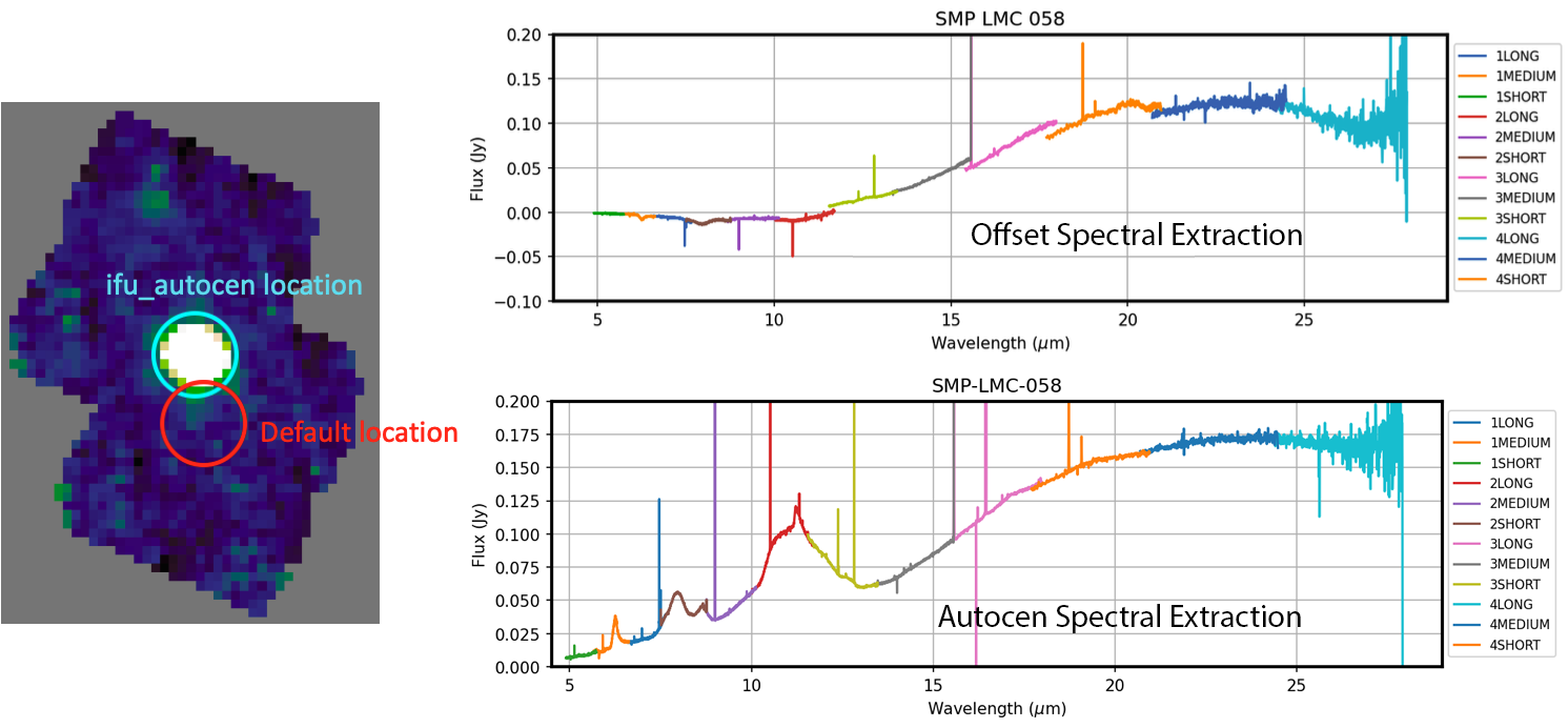
Click on the figure for a larger view.
Left panel: In this case (Program ID 1523, Observation 3) the embedded WCS provided by the telescope attitude information was initially incorrect by about 1.3", resulting in a 1-D spectral extraction aperture that missed the source entirely. As a result (right panel) the extracted spectrum was near zero or slightly negative at short wavelengths due to the presence of the source in the annular background region. At longer wavelengths the miscentering was less important due to the increasing size of the aperture extraction region. In contrast to the coordinate-based extraction, the auto-centroiding option does a good job of finding the source and extracting in the correct location.
Summary of common issues and workarounds
The sections above provide details on each of the known issues affecting MRS data; this table summarizes some of the most likely issues that users will encounter along with any workarounds if available. Note that greyed-out issues have been retired, and are fixed as of the indicated pipeline build.
| Symptoms | Cause | Workaround | Fix Build | Mitigation Plan |
|---|---|---|---|---|
Data cubes show repeating bright/dark artifacts in the data cubes. See Bad Pixels section above. | Bad pixels on the detector can produce artifacts in the final data cubes | A notebook exists to use dedicated background data to create a custom bad pixel mask for individual science programs: see MRS_Flag_Badpix.ipynb | N/A | January 2024 saw a major update to the bad pixel flagging to implement variable flagging for different exposure depths and regular updates to the mask. New bad pixels will always occur however, and the workaround notebook may be implemented as an optional step in the pipeline in future. |
MR-MRS04: Spectra show residual regular periodic amplitude modulations. See Fringing section above. | MRS experiences significant spectral fringing, which varies with the astronomical scene and cannot be automatically corrected in its entirety for all science targets. | Run the 2-D or 1-D (preferred) residual_fringe correction steps available in the pipeline (jwst 1.11.0 onwards). This is discussed in greater detail in the Fringing section above. | N/A | Created issue None; additional non-default corrections are science case specific. Calibrations programs will explore possible future mitigations. |
MR-MRS05: Spectra extracted from small spatial regions show amplitude modulations of variable frequency (distinct from ordinary spectral fringes). See Resampling section above. | The MRS is not Nyquist sampled, and resampling the raw data to a rectified data cube introduces artifacts if extracting spectra on scales smaller than the PSF. See detailed discussion by Law et al. 2023. | Extract spectra from apertures comparable to PSF in width. | N/A | Created issue This is still under investigation; some science cases may permit scene modeling to mitigate impact. |
| MR-MRS06: The "ERR" extension in "rate" data products (and other error estimates downstream) is incorrect, sometimes by factors of 10–50. See Variance section above. | Error values are estimated incorrectly by the pipeline. | Bootstrap uncertainty from science spectra, being careful to eliminate residual fringing first. | N/A | Created issue The root cause of incorrect error estimates in the pipeline is being investigated. |
| MR-MRS01: World coordinate system (WCS) of data cubes is incorrect. See WCS Accuracy section above. | WCS is typically incorrect by 0.3" and in some cases more than 1" due to incorrect guide star information. | None. | N/A |
Investigate providing a notebook to update MRS WCS based on simultaneous imaging data. |
| MR-MRS03: Spectra show unexpected features around 12.2 µm. See Spectral Leak section above. | There is a spectral leak in the MRS where a small amount of light from 6 µm is received by the 12 µm channel. | A notebook is available to to apply a correction for the MRS spectral leak to point source data. | Updated issue A correction step has been included in pipeline version 1.13.0 and later for point source data. No correction is available for extended sources as the 12 µm and 6 µm channels have different spatial footprints. | |
| MR-MRS08: Channel 4B field of view is squashed by about 8% relative to the 4A and 4C fields. This is noticeable in observations of sources with fixed limbs comparable in size to the FOV (e.g., giant planets). | Channel 4B distortion solution was incorrect due to limitations in the astrometric calibration. | New 4B distortion solution has been derived that fixes the issue and will be available shortly in CRDS. | Updated Operations Pipeline New reference files and jwst_1125.pmap context were delivered to Operations Pipeline; reprocessing of affected data typically takes 2–4 weeks after the update. | |
| Extracted flux from a point source can be much fainter than expected or negative. See Spectral Extraction section above. | WCS is typically incorrect by 0.3" and in some cases more than 1". Spectral extraction aperture is centered on target coordinates assuming WCS is correct. | Install the latest release of the jwst package and then run the Science Calibration Pipeline on the affected dataset. Starting in jwst 1.11.0, the extract_1d step supports setting ifu_autocen = True. (JP-3011) | Updated Operations Pipeline DAOStarFinder is used to locate point sources in the image constructed from the collapsed 3-D cube. Proper motion is now applied correctly. STScI reprocessed affected data products with an updated Operations Pipeline that was installed on August 24, 2023. ()Reprocessing of affected data typically takes 2–4 weeks after the update. STScI plans to provide software that updates the MIRI MRS WCS based on simultaneous imaging data. An availability date is to be determined. | |
| MR-MRS02: The photon count rate and derived flux is lower than predicted at long wavelengths, with maximum deficit roughly a factor of 2 at 28 µm. See Count Rate Loss section above. | MRS sensitivity at long wavelengths is decreasing with time. | Use the new Science Calibration Pipeline software (jwst 1.11.0 onwards) to apply the time-dependent throughput correction, using new reference data (jwst_1094.pmap onwards). This is available as of . (JP-3224) | Updated Operations Pipeline Only for non-TSO data: new time-dependent throughput corrections were applied. STScI reprocessed affected data products with an updated Operations Pipeline that was installed on August 24, 2023. (Reprocessing of affected data typically takes 2–4 weeks after the update.) See this JWST Observer new item for more details. Fixed for TSO data in Build 10.0 |
References
Argyriou, I., et al. 2020, A&A, 641, A150 (MRS Fringing)
The nature of point source fringes in mid-infrared spectra acquired with the James Webb Space Telescope
Argyriou, I., et al. 2023, A&A, 675, A111 (MRS Overview)
JWST MIRI flight performance: The Medium-Resolution Spectrometer
Kavanagh, P., et al. 2023, in prep
Law, D. R., et al. 2023, AJ, 166, 45 (MRS Cube Building)
A 3D Drizzle Algorithm for JWST and Practical Application to the MIRI Medium Resolution Spectrometer