JWST Fine Guide Stability
JWST's line-of-sight stability, based on actual performance, data products for the Fine Guidance Sensors, and measuring jitter during an observation are covered in this article.
On this page
Guiding precision and pointing stability
For fixed targets, pointing stability is evaluated as the rms error in the guide star position in a 15 s interval, compared to the mean position over a 10,000 s observation.
Line-of-sight (LOS) pointing stability under fine guiding control is excellent. The Fine Guiding Sensor (FGS) sensing precision is parameterized as the noise equivalent angle (NEA, an equivalent jitter angle based on centroid position and SNR), and is usually ~1 mas (1-σ per axis), symmetric. The LOS jitter seen in the science instruments is similarly good, and high frequency sampling of the jitter in a NIRCam small subarray is the same, ~1 mas (1-σ per axis). Although a drift in observatory roll could theoretically generate image drift in a long duration observation, experience indicates such drifts while in fine guide control are negligible.
For Solar System (moving) targets, the line-of-sight pointing stability is evaluated as the rms value over a 1,000 s observation for a linear motion of 3.0 mas/s, and is estimated to be 6.2 to 6.7 mas (1-σ per axis, depending on the science instrument).
If you have reason to doubt the accuracy of the guiding for your science data, one thing you could do is to inspect the calibrated fine guide images. The sections below detail how to retrieve the guiding data from MAST, the naming conventions and contents of the guiding data, details about available jitter data, as well as obtaining information on the guide stars and reference stars and tools to analyze jitter data.
JWST Fine Guidance Sensor data products
See also: Guide Star Data Products (documentation external to JDox)
The FGS has several modes, as explained on the Fine Guidance Sensor article. Each mode produces different data products, with the characteristics listed below.
Correlated double sample (CDS) images
Correlated double sample (CDS) images are computed onboard, and in the guide star pipeline, for ID, ACQ, and TRACK mode images. In this technique, the readout pattern is two integrations, each with two reads: RESET, READ, READ; RESET, READ, READ. Each integration begins with a RESET. The first read of each integration is the pedestal-1 image; the second read of each integration is the signal-1 image. The CDS1 image is signal-1 – pedestal-1. Subtracting the pedestal image from the signal image removes the pedestal bias on a pixel-by-pixel basis. Thus, from four readouts you will obtain two CDS images, CDS1 and CDS2.
In order to understand the details of the guiding performance for a particular set of science observations, a user may want to do download, inspect, and/or analyze the JWST guide star products from the archive. Below are step by step instructions for how to do this.
Retrieving guiding data from MAST
The following Python snippet shows an example of how to retrieve guiding data from MAST. This assumes that an appropriate Python environment has been set up that includes the packages astroquery, and requests. For other ways of getting the data, see Accessing JWST Data. For more details about programmatic access, see MAST API Access.
from astroquery.mast import Mast
import os
from requests.exceptions import HTTPError

# To create a new API token visit the following link:
# https://auth.mast.stsci.edu/token?suggested_name=Astroquery&suggested_scope=mast:exclusive_access
tkn = 'abcdefghijklmnopqrstuvwxyz012345' # enter your new API token here
visit_id = 'jw01234567890'               # enter your visit id (jwppppvvvooo) here

server = "https://mast.stsci.edu/"
output_path = None
redownload = False
indir = os.getcwd() + '/'
os.chdir(indir)

# retrieve level-2-calibrated ID, ACQ, TRACK, and FG data
params = {"columns":"*",
          "filters": [
              {"paramName": "fileSetName",
               "values": [visit_id+'_gs-id', visit_id+'_gs-acq1', visit_id+'_gs-acq2', visit_id+'_gs-track', visit_id+'_gs-fg']},
              {"paramName": "productLevel",
               "values": ['2','2','2','2','2']}
          ]}

Mast.login(token = tkn)
print('asking for table')
table = Mast.service_request('Mast.Jwst.Filtered.GuideStar', params)
filenames = table['fileName']
print(filenames)

output_path = indir + visit_id + '/'
if output_path is None:
    output_path = '.'
else:
    output_path = output_path

for ifile in filenames:
    output_filename = os.path.join(output_path, ifile)
    if not os.path.exists(output_path):
        os.mkdir(output_path)
    if os.path.exists(output_filename) and not redownload:
        print(f"Found file previously downloaded: {ifile}")
    data_uri = f'mast:JWST/product/{ifile}'

    print('downloading files')
    url_path = Mast._portal_api_connection.MAST_DOWNLOAD_URL
    try:
        Mast._download_file(url_path + "?uri=" + data_uri, output_filename)
    except HTTPError as err:
        print(err)
    print(output_filename)
Guiding data products naming conventions
In the sections below, the following shorthand is used in describing the guiding data file names:
- ‘jw’ is the mission identifier for JWST data
- <ppppooovvv> is the visit id and contains the proposal id (pppp), the observation number (ooo), and the visit id (vvv)
- <m> is the guide star Identification attempt number; this can range from 1 to 9
- The timestamp <yyyydddhhmmss> is the year (yyyy), day of year number (ddd), hour (hh), minute (mm), and seconds at the end of the data in the file. The timestamp is used to differentiate between multiple instances of these files in a single visit
Guiding data products contents
See also: Guide Star Data Products (documentation external to JDox)
The contents of the data products are detailed in the following tables.
Identification (ID) mode data products
ID data is not in closed loop guiding. Users should not attempt to use ID data for WCS information.
ID mode data products include stream, unstacked uncal & cal, and stacked uncal & cal files. Stream and uncal data are not typically used for science. Table 1 gives the naming convention and extension contents for the data products. <pppppooovvv> is the program id, observation number, and visit number. <m> is the guide star identification attempt within a visit (m = 1-9).
Table 1. Filenames and extension contents for ID data products
File type | Extension # | Name & type |
|---|---|---|
ID stream jw<pppppooovvv>_gs-id_<m>_stream.fits | 0 1 2 3 | |
ID image_uncal jw<pppppooovvv>_gs-id_<m>_image-uncal.fits | 0 1 2 3 4 | PRIMARY Header SCI Image (2024, 2048, 2, 2) FLIGHT REFERENCE STARS BinTable * PLANNED REFERENCE STARS BinTable ASDF BinTable |
ID stacked_uncal jw<pppppooovvv>_gs-id_<m>_stacked-uncal.fits | 0 1 2 3 4 | ASDF BinTable |
ID image_cal jw<pppppooovvv>_gs-id_<m>_image-cal.fits | 0 1 2 3 4 5 6 | PRIMARY Header SCI Image (2024, 2048,1) ERR Image (2024, 2048,1) DQ Image (2024, 2048) PLANNED REFERENCE STARS BinTable FLIGHT REFERENCE STARS BinTable * ASDF BinTable |
ID stacked_cal jw<pppppooovvv>_gs-id_<m>_stacked-cal.fits | 0 1 2 3 4 5 6 | PRIMARY Header SCI Image (2304, 2048, 1) ERR Image (2304, 2048, 1) DQ Image (2304, 2048) PLANNED REFERENCE STARS BinTable FLIGHT REFERENCE STARS BinTable * ASDF BinTable |
* Flight Reference Stars binary table was not populated correctly prior to August 21, 2025.
Crowded field data products
Only stars that make it onto the bright object list during Identification may be considered as guide star candidates. In bright crowded fields, there are too many bright stars in the guider's field of view and the bright object list fills up before the entire detector can be read. Consequently, for bright crowded fields, only the central third of the detector is read out. This increases the chances that the commanded guide star and reference stars make it onto the bright object list, which is limited to 100 objects. The overall dimensions of the data files are the same as above, with the portion of the detector that was not read out set to 0.
Acquisition 1 (ACQ1) mode data products
ACQ1 data is not in closed loop guiding. Users should not attempt to use ID data for WCS information.
ACQ1 mode data products include stream, uncal & cal files. Stream and uncal data are not typically used for science. Different attempts at ACQ are differentiated by the timestamps embedded in the file names. Table 2 gives the naming convention and the extension contents for the ACQ1 data products. <pppppooovvv> is the program id, observation number, and visit number. <yyyydddhhmmss> is the time stamp at the end of data contained in the file.
Table 2. Filenames and extension contents for ACQ1 data products
File type | Extension # | Name & type |
|---|---|---|
ACQ1 stream jw<pppppooovvv>_gs-acq1_<yyyydddhhmmss>_stream.fits | 0 1 | PRIMARY Header SCI Image (128, 128, NAXIS3) |
ACQ1 uncal jw<pppppooovvv>_gs-acq1_<yyyydddhhmmss>_ uncal.fits | 0 1 2 | PRIMARY Header SCI Image (128, 128, 2, 6) ASDF BinTable |
ACQ1 cal jw<pppppooovvv>_gs-acq1_<yyyydddhhmmss>_ cal.fits | 0 1 2 3 4 | PRIMARY Header SCI Image (128, 128, 6) ERR Image (128, 128, 6) DQ Image (128, 128) ASDF BinTable |
Acquisition 2 (ACQ2) mode data products
ACQ2 data is not in closed loop guiding. Users should not attempt to use ID data for WCS information.
ACQ2 mode data products include stream, uncal & cal files. Stream and uncal data are not typically used for science. Different attempts at ACQ are differentiated by the timestamps embedded in the file names. Table 3 gives the naming convention and extension contents for the ACQ2 data products. <pppppooovvv> is the program id, observation number, and visit number. <yyyydddhhmmss> is the time stamp at the end of data contained in the file.
Table 3. Filenames and extension contents for ACQ2 data products
File type | Extension # | Name & type |
|---|---|---|
ACQ2 stream jw<pppppooovvv>_gs-acq2_<yyyydddhhmmss>_stream.fits | 0 1 | PRIMARY Header SCI Image (32, 32, 10) |
ACQ2 uncal jw<pppppooovvv>_gs-acq2_<yyyydddhhmmss>_ uncal.fits | 0 1 2 | PRIMARY Header SCI Image (32, 32, 2, 5) ASDF BinTable |
ACQ2 cal jw<pppppooovvv>_gs-acq2_<yyyydddhhmmss>_ cal.fits | 0 1 2 3 4 | PRIMARY Header SCI Image (32, 32, 5) ERR Image (32, 32, 5) DQ Image (32, 32) ASDF BinTable |
Track mode data products
Track mode data products include stream, uncal and cal files. Stream and uncal data are not typically used for science. Different attempts at TRACK are differentiated by the timestamps embedded in the file names. Table 4 gives the naming convention and extension contents for the Track data products. <pppppooovvv> is the program id. <yyyydddhhmmss> is the time stamp at the end of data contained in the file.
Table 4. Filenames and extension contents for track data products
File Type Naming Convention | Extension # | Name & type |
|---|---|---|
TRACK stream jw<pppppooovvv>_gs-track_<yyyydddhhmmss>_stream.fits | 0 1 | PRIMARY Header SCI Image (32, 32, NAXIS3) |
TRACK uncal jw<pppppooovvv>_gs-track_<yyyydddhhmmss>_ uncal.fits | 0 1 2 3 4 5 | PRIMARY Header SCI Image (32, 32, 2, NAXIS4) ASDF BinTable |
TRACK cal jw<pppppooovvv>_gs-track_<yyyydddhhmmss>_ cal.fits | 0 1 2 3 4 5 6 7 | PRIMARY Header SCI Image (32, 32, NAXIS3) ERR Image (32, 32, NAXIS3) DQ Image (32, 32) ASDF |
Fine guide (FG) data products
Fine guide mode data products include stream, uncal and cal files. Stream and uncal data are not typically used for science. Different attempts at fine guide are differentiated by the timestamps embedded in the file names. Table 5 gives the naming convention and extension contents for the fine guide data products. <pppppooovvv> is the program id. <yyyydddhhmmss> is the time stamp at the end of data contained in the file.
Table 5. Filenames and extension contents for fine guide data products
File type | Extension # | Extension Type | Name & type |
|---|---|---|---|
FG stream jw<pppppooovvv>_gs-fg_<yyyydddhhmmss>_stream.fits | 0 1 | Header Image | PRIMARY Header SCI Image (8, 8, NAXIS3) |
FG uncal jw<pppppooovvv>_gs-fg_<yyyydddhhmmss>_ uncal.fits | 0 1 2 3 4 | Header Image BinTable BinTable BinTable | |
FG cal jw<pppppooovvv>_gs-fg_<yyyydddhhmmss>cal.fits | 0 1 2 3 4 5 6 | Header Image Image Image BinTable BinTable BinTable | PRIMARY Header SCI Image (8, 8, NAXIS3) ERR Image (8, 8, NAXIS3) DQ Image (8, 8) ASDF BinTable |
Some guide data files are split into multiple segments; if this is the case, all of the segmented guiding files for the guiding period in question should be retrieved from MAST and the data should be concatenated. See Segmented Products for more information.
Guide star and reference star information
The "stacked_cal", and "image_cal" Identification data files provide information on the planned and used guide stars and reference stars. For details, see Guide Star and Reference Star Information.
Jitter data products
Stream (jwpppppvvvooo_gs-track_*_stream.fits) and uncal (jwpppppvvvooo_gs-track_*_uncal.fits) files are typically not used for science or jitter analysis. Use cal files (jwppppvvvooo_gs-fg_*_cal.fits) for jitter analyses.
The jitter is defined at the reference pixel position as √((delta(DDC RA))2 + (delta(DDC Dec))2). The DDC is the differential distortion compensation field point, which corresponds to a specific location in the science instrument aperture. The attitude control system optimizes the pointing at the DDC field point by determining how to command the fine steering mirror and minimizing the jitter at that point, rather than at the guide star in the FGS.
TRACK and FINE GUIDE mode data products capture a FITS table extension for jitter data. The table data will capture the differences between the reference value of a pointing parameter and the value at every sampled time in the data file. The reference value is determined by taking the average value of each parameter, excluding the settling time.
The pointing table extension contains the following jitter keywords:
JITTRMIN: the minimum value of the jitter over the duration of the data fileJITTRMAX: the maximum value of the jitter over the duration of the data fileJITTRAVG: the average value of the jitter over the duration of the data file
Note: Data values throughout the settling time should not be included in the determination of statistical jitter values.
POINTING Table Columns
Table 6 below shows the content of the track and fine guide POINTING tables.
Table 6. Content of POINTING table for track and fine guide data
| POINTING table field | Units | Description |
|---|---|---|
| Time | miliiseconds | Time since start time of data file |
| Jitter | milliarcseconds | √( (delta(DDC RA))2 + (delta(DDC Dec))2 ) |
| Delta DDC RA | milliarcseconds | Difference between current and initial DDC RA |
| Delta DDC Dec | milliarcseconds | Difference between current and initial DDC Dec |
| Delta Aper PA | milliarcseconds | Difference between current and initial aperture PA |
| Delta V frame RA | milliarcseconds | Difference between current and initial V frame RA |
| Delta V frame Dec | milliarcseconds | Difference between current and initial V frame Dec |
| Delta V frame PA | milliarcseconds | Difference between current and initial V frame PA |
| Delta J frame RA | milliarcseconds | Difference between current and initial J frame RA |
| Delta J frame Dec | milliarcseconds | Difference between current and initial J frame Dec |
| Delta J frame PA | milliarcseconds | Difference between current and initial J frame PA at J1 |
| HGA motion | N/A | HGA state: 0 = MOVING; 1 = FINISHED; 2 = OFFLINE |
CENTROID PACKET table columns
Table 7 shows the content of the CENTROID PACKET tables for track and fine guide data
Table 7. Content of CENTROID table for track and fine guide data
| CENTROID table field | Units | Description |
|---|---|---|
| observatory_time | UTC YYYY/MM/DD HH:MM:SS.mmm | UTC time defined by the Eclipse setup of the Observatory time when the packet containing this value was generated |
| centroid_time | seconds | Seconds since 2000-001/00:00:00 |
| guide_star_position_x | arc-sec | FGS Ideal frame |
| guide_star_position_y | arc-sec | FGS Ideal frame |
| guide_star_instrument_counts_per_sec | counts/sec | 3x3 pixel count sum per second |
| signal_to_noise_current_frame | no units | Signal/Noise for current image frame TRK & FG: (signal/noise)/100.0 |
| delta_signal | scaled counts | Scaled signal difference between current and previous frame TRK & FG: abs(signal1-signal2)/700. |
| delta_noise | scaled counts | Scaled noise difference between current and previous frame TRK: abs(noise1-noise2)/3.0 FG: abs(noise1-noise2)/12.0 |
| psf_width_x | pixels | Width of PSF in ideal x direction |
| psf_width_y | pixels | Width of PSF in ideal y direction |
| data_quality | no units | Centroid data quality |
| bad_pixel_flag | GOOD/BAD | Bad pixel status for detector subwindow |
| bad_centroid_dq_flag | GOOD/BAD | Centroid data quality flag (1 = bad centroid) |
| cosmic_ray_hit_flag | YES/NO | Computed from avg of last few frames |
| sw_subwindow_loc_change_flag | YES/NO | Software subwindow location change flag |
| guide_star_at_detector_boundary_flag | YES/NO | Guide star at detector boundary flag |
| subwindow_out_of_FOV_flag | YES/NO | Subwindow out of FOV flag |
TRACK SUBARRAY table columns
Table 8 shows the content of the TRACK SUBARRAY table for track data
Table 8. Content of TRACK SUBARRAY table for track data
| TRACK SUBARRAY table field | Units | Description |
|---|---|---|
| observatory_time | UTC YYYY/MM/DD HH:MM:SS.mmm | UTC time defined by the Eclipse setup of the Observatory time when the packet containing this value was generated |
| x_corner | arc-sec | subarray x-axis corner in ideal coordinate frame |
| y_corner | arc-sec | subarray y-axis corner in ideal coordinate frame |
| x-size | pixels | size of subarray x-axis |
| y-size | pixels | size of subarray y-axis |
Measuring jitter
Jitter is measured at the position of the guide star in the FGS, then mapped to the differential distortion compensation field point specified in the engineering telemetry. Jitter data is available in the "Pointing " table extension for track and fine guide data FITS files. Use cal files (jwppppvvvooo_gs-fg_*_cal.fits) for jitter analyses.
If you wish to investigate the guiding for your science data, you could plot the "jitter ball." Below are some sample lines of Python code that show how to do this for files retrieved from MAST.
from astropy.table import Table
import astropy.io.fits as fits
import astropy.time
import numpy as np
import matplotlib, matplotlib.pyplot as plt

sci_file = '/path/name/to/your/science_cal_file.fits'
guide_file = '/path/name/to/your/guiding_cal_file.fits'

# read science exposure beginning and end times from science data
with fits.open(sci_file) as sci_hdul:
    t_sci_beg = astropy.time.Time(sci_hdul[0].header['DATE-BEG'])
    t_sci_end = astropy.time.Time(sci_hdul[0].header['DATE-END'])

# read centroid data from guiding data
with fits.open(guide_file) as guide_hdul:
    centroid_table = astropy.table.Table.read(guide_hdul, hdu=5)
    ctimes = astropy.time.Time(centroid_table['observatory_time'])

# disregard centroids marked by the FSW as "BAD"
mask = centroid_table.columns['bad_centroid_dq_flag'] == 'GOOD'

# determine the centroids that are during the science exposure
during_exp = (t_sci_beg < ctimes[mask]) & (ctimes[mask] < t_sci_end)

# calculate mean of centroids in X & Y
xmean = np.nanmean(centroid_table[mask]['guide_star_position_x'])
ymean = np.nanmean(centroid_table[mask]['guide_star_position_y'])

# calculate offsets of centroids from mean position & convert to milli-arc-seconds
x = (centroid_table[mask][during_exp]['guide_star_position_x'] - xmean) * 1000.
y = (centroid_table[mask][during_exp]['guide_star_position_y'] - ymean) * 1000.

# calculate the standard deviations of the centroid offsets in X & Y
std_x = x.std()
std_y = y.std()
print("Standard deviation in X = "+str(std_x)+" mas")
print("Standard deviation in Y = "+str(std_y)+" mas")

# plot jitter ball
plt.plot(x, y, '+')
plt.title("Jitter")
plt.xlabel("GS Centroid Offset X (mas)")
plt.ylabel("GS Centroid Offset Y (mas)")
plt.show()
Figure 2. Jitter measurements from a calibration observation (PID 4495, observation 2)
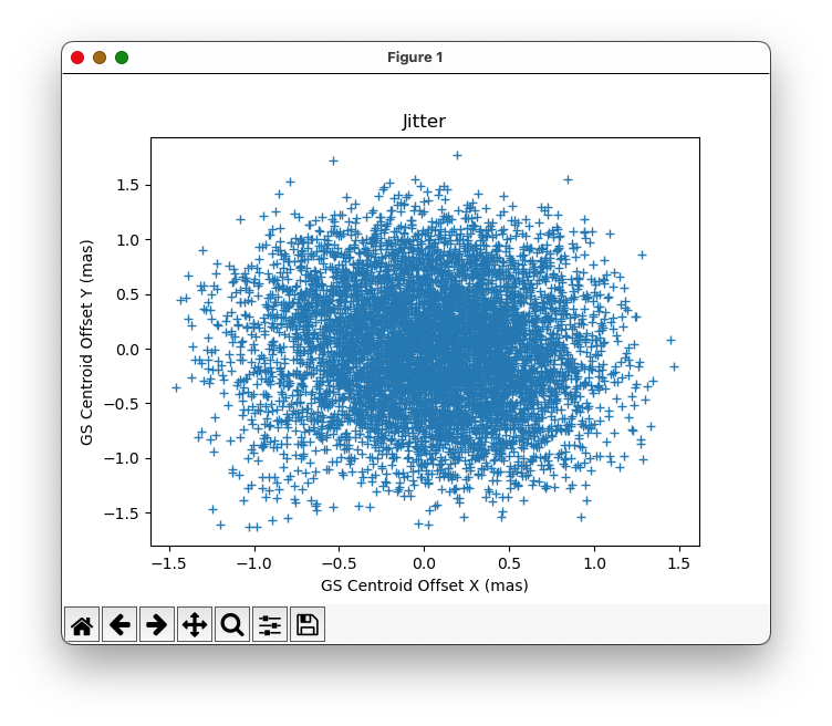
Example of a "jitter ball" plot
Jitter tools
JWST FGS Spelunker (Deal & Espinoza) is an FGS quick-look pipeline package that provides an easy-to-access ("plug-and-play") library to access this guide star data. Generate time-series for several metrics of the FGS data in an automated fashion, including fluxes and PSF variations.
References
Deal, D. and Espinoza, N., 2024, JOSS, 9(97), 6202
Spelunker: A quick-look Python pipeline for JWST NIRISS FGS Guide Star Data