JWST Multistripe, Superstripe, and Substripe Detector Modes
The JWST "multistripe" detector mode can read disjoint regions on the detector ("substripe") and map a region by shifting a smaller subarray ("superstripe").
On this page
Overview
See also: NIRCam Multistripe Subarrays for Grism Time Series Spectroscopy, NIRCam Superstripe Subarrays for Imaging and Time Series Imaging, NIRISS Detector Readout, NIRISS Detector Subarrays, NIRSpec Detector Subarray Mode
In Cycle 4, JWST started rolling out a new "multistripe" detector readout mode to some near-infrared instrument templates. Multistripe makes it possible to read disjoint regions of the detector in a single frame ("substripe") and/or to cover a larger detector region with a shifting sequence of smaller subarray integrations ("superstripe"). Multistripe can read reference pixels at the detector edge and interior science pixels, skipping the intervening rows. Superstripe integrations are quicker than normal subarray integrations, so brighter targets can be observed without saturation, but note that signal collected per pixel is reduced by a large factor relative to a normal exposure with comparable execution time.
Superstripe should only be used when a target is too bright for a normal subarray.
Templates with multistripe options
Starting in Cycle 4, the NIRCam grism time-series mode template offered spectroscopy in the short wavelength channel, using the Dispersed Hartmann Sensor (DHS). The DHS directs light collected by different regions of the primary mirror to different locations on the detector, producing regularly spaced spectra. DHS substripe efficiently reads and packages these disjoint spectra into each frame.
Starting in Cycle 5, the NIRISS SOSS template offered SOSS superstripe subarrays.
Starting in Cycle 6, the NIRSpec bright object time-series mode template offered prism superstripe subarrays. In addition, the NIRCam imaging and imaging time-series templates offered NIRCam imaging superstripe subarrays.
Multistripe design
For context, the simplest JWST exposure is a loop over contiguous detector rows, nested inside a loop over frames that cover the same rows, nested inside a loop over integrations. For a subarray, the contiguous rows may be a subset of all detector rows. Frames are combined into groups as specified by the selected readout pattern. Each integration consists of a reset followed by multiple reads of each pixel as charge accumulates. Schematically:
- Loop over integrations in an exposure
- Loop over frames in an integration; combine frames into groups; write groups to the recorder
- Loop over a set of contiguous detector rows; package rows into a frame
- Loop over frames in an integration; combine frames into groups; write groups to the recorder
Multistripe adds two additional layers of nesting via additional multistripe control parameters. Schematically:
- Loop over integrations in an exposure
- Loop over "superstripe integrations" in an integration
- Loop over frames in a superstripe integration; package frames into groups; write groups to the recorder
- Loop over reference pixel rows and substripes in a frame; package rows into a frame
- Loop over detector rows in a substripe
- Loop over reference pixel rows and substripes in a frame; package rows into a frame
- Loop over frames in a superstripe integration; package frames into groups; write groups to the recorder
- Loop over "superstripe integrations" in an integration
Detector rows may appear as image columns in a science data product, if the image has been reoriented (SLOWAXIS = 2 in the FITS header).
Reference pixel rows
Multistripe exposures can read reference pixel rows before reading the first set of science pixel rows (stripe) and optionally between substripes in a frame. The Reads1 parameter specifies how many reference pixel rows to read. If Reads1 = 0, no reference pixel rows are read. The RowCorner parameter (also used for normal subarrays) specifies the first detector row in the subarray and hence the first reference pixel row to read in a multistripe subarray. If RowCorner = 1, the first reference pixel row is at the edge of the detector. For example, RowCorner = 1 and Reads1 = 4 reads all four reference pixel rows at the edge of the detector.
In principle, "reference pixel rows" could include normal science pixel rows (if RowCorner + Reads1 > 4), but in practice Reads1 is only used to read reference pixel rows. For expository convenience in this article, we reserve the term "substripe" (see next section) for a contiguous set of science pixel rows and explicitly use "reference pixel rows" when referring to the contiguous set of reference pixel rows specified by RowCorner and Reads1.
Substripes
A single frame in a multistripe exposure contains one or more substripes. If an exposure is not using superstripe (see next section and Figure 1), then there are Skips1 skipped rows between the reference pixel rows and the first substripe in a frame. The first substripe in a frame may be adjacent to the reference pixel rows (Skips1 = 0) or disjoint (Skips1 > 0), but the two regions may not overlap (Skips1 < 0 is not allowed).
Each substripe in a frame contains the same number of science pixel rows (Reads2). Substripes in a frame are regularly spaced. The row offset between the start of consecutive substripes in a frame is either 0 (if Repeat = 1 and Interleave = 0, see below) or Skips2. Substripes can cover disjoint regions on the detector (Skips2 > Reads2), adjacent regions (Skips2 = Reads2), overlapping regions (Skips2 < Reads2), or identical regions (Repeat = 1 and Interleave = 0, or alternatively Skips2 = 0).
Figure 1 shows how the Repeat and Interleave parameters control the behavior of substripes. The Interleave parameter is only meaningful when Repeat = 1.
- When Repeat = 0 (left column of Figure 1), reference pixel rows (Reads1) are read only once per frame at the beginning of the frame, the offset between the start of each substripe is Skips2, and substripes are read until the frame is filled.
- When Repeat = 1 and Interleave = 0 (middle column of Figure 1), reference pixel rows are read before every substripe and the same set of science pixel rows are read in every substripe until the frame is full. Charge accumulates in pixels between each substripe read, so a single frame contains up-the-ramp measurement like an integration, but the data are packaged into a single frame. NIRCam Grism Time Series subarrays use this configuration in the long-wavelength channel to gather useful data while short-wavelength channel is reading multiple DHS stripes.
- When Repeat = 1 and Interleave = 1 (right column of Figure 1), reference pixel rows are read before every substripe, the offset between the start of each substripe is Skips2, and substripes are read until the frame is filled. NIRCam Grism Time Series subarrays use this configuration in the short-wavelength channel to read and package multiple DHS stripes into a single frame.
Figure 1. Schematic showing the three substripe configurations
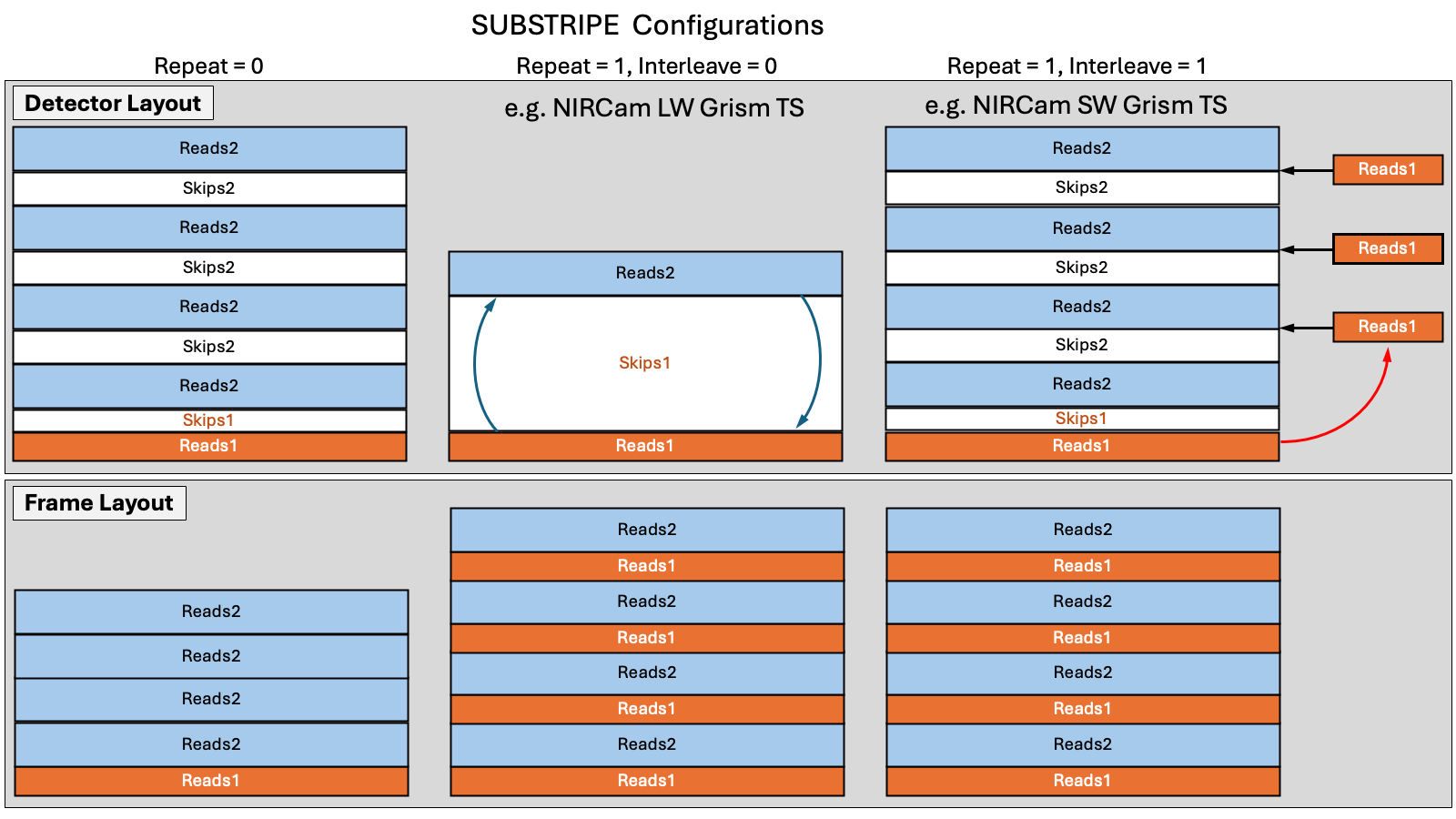
Click on the figure for a larger view.
Notional placement and sizes of reference pixel rows and substripes in the three substripe configurations (left, middle, and right columns). The top part of the figure shows where the reference pixel rows and substripes are located on the detector. The bottom part of the figure shows how reference pixel rows and substripes are packaged into a single frame. See text for a discussion of the relevant multistripe parameters that control substripe.
- (Nrow - Reads1) / Reads2, if reference pixel rows are only read once at the start of a frame (Repeat = 0, left column in Figure 1)
- Nrow / (Reads1 + Reads2), if reference pixel rows are read before every substripe (Repeat = 1, middle and right columns in Figure 1)
Superstripes
Each normal integration in a multistripe exposure can contain multiple superstripe integrations (or more concisely "superstripes"). Each superstripe integration generates multiple frames that record charge accumulating up-the-ramp in a subset of detector rows. Frames are combined into groups and sent to the recorder for eventual downlink. Detector rows in each frame may include reference pixels and multiple substripes, though in practice superstripe subarrays currently have only one substripe per frame and may also include reference pixel rows.
Multistripe splits each normal integration into a number of superstripes (Nsuper). The science rows in each successive superstripe are offset by a number of rows (Superstep) from science rows in the preceding superstripe. The general formula for the first science pixel row in a superstripe is:
First Science Row = RowCorner + Reads1 + Skips1 + Isuper * Superstep,
where Isuper is a superstripe index that runs from 0 to Nsuper - 1 within a normal integration. For example, a detector region with 2040 science rows (e.g., the full NIRISS SOSS spectrum) could be fully covered by four superstripes (Nsuper = 4), each measuring charge accumulation in 510 science rows (Reads2 = 510) with an offset of 510 rows between each superstripe integration (Superstep = 510). The first science row in each superstripe would be 5, 515, 1025, and 1535, where row index here ranges from 1 to 2048.
Superstripes can cover disjoint regions on the detector (e.g., Superstep > Reads2), adjacent regions (Superstep = Reads2), overlapping regions (Superstep < Reads2), or identical regions (Superstep = 0). Currently, all multistripe subarrays that use superstripe have adjacent superstripes (Superstep = Reads2). Figure 2 shows this superstripe geometry.
All detector rows are reset at the start of each superstripe integration. Because each superstripe covers a subset of detector rows (e.g., 510 vs. 2040), frame times are shorter and so brighter sources can be observed without saturating. However, signal accumulating in other superstripe regions is reset without being measured, so overall observing efficiency is reduced by a factor of approximately Nsuper. Because of this large reduction in efficiency, superstripe should only be used for sources that are too bright to observe any other way. For example, see the detector decision flowchart for BOTS observations on the NIRSpec Detector Recommended Strategies page.
Figure 2. Schematic showing a superstripe exposure
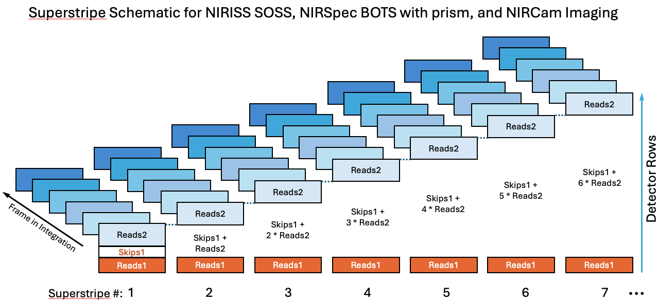
Click on the figure for a larger view.
Notional placement and sizes of reference pixel rows and superstripes in one normal integration. The integration is split into 7 superstripe integrations that execute sequentially from left to right in the figure. Each superstripe integration contains 6 frames that are read front to back in the figure. The darker color in each successive frame indicates that charge is accumulating over the course of the superstripe integration. All detector rows are reset when switching from one superstripe to the next. Reference pixel rows (labelled Reads1 in the figure) are read at the start of every frame, but the figure only shows reference pixels for the first frame to avoid visual clutter.
Nomenclature
In general, a single multistripe exposure can read reference pixel rows, multiple substripes in a frame, and multiple superstripes. In practice, it is useful to distinguish between two common cases that use subsets of the full suite of multistripe capabilities:
- A "substripe exposure" reads multiple substripes per frame, but only one superstripe. Each frame may include reference pixel rows, as well. Substripe exposures are useful for combining disjoint sets of science rows into a single frame. NIRCam Grism Time Series uses this capability to combine multiple DHS spectra into each short-wavelength frame.
- A "superstripe exposure" has multiple superstripes, but reads only one substripe per frame. Each frame may include reference pixel rows, as well. Superstripe exposures enable observations of brighter targets without saturation by splitting a large detector area into smaller areas, each with a shorter frame time. The shorter frame time makes it possible to observe brighter targets without saturation. NIRISS SOSS, NIRSpec BOTS with the prism, and NIRCam Imaging all have superstripe subarrays.
It is correct to use the generic term "multistripe exposure" for a substripe exposure or a superstripe exposure, but the more specific terms help communicate why multistripe is being used for a specific application.
Multistripe control parameters
Observers cannot explicitly specify multistripe control parameters. Instead, observers can choose a multistripe subarray in some APT templates. Each multistripe subarray definition includes pre-defined values for each multistripe control parameter, which are ultimately reported in header keywords in data products (see tables below). The detail provided here is intended to provide a basic understanding of how multistripe exposures operate "under the hood".
Each JWST near-infrared detector is controlled by its own SIDECAR Application Specific Integrated Circuit (ASIC). All JWST SIDECARs have the same hardware design and run the same firmware, which is occasionally updated. During an exposure, a SIDECAR addresses and reads a range of detector columns in one detector row before proceeding to another detector row. Because of this nesting, the loop over columns is called the "fast" readout direction and the loop over rows is called the "slow" readout direction. Multistripe only affects which rows are read and the sequence in which they are read, so every stripe covers exactly the same columns.
One multistripe parameter (Reads1) and one normal subarray parameter (RowCorner) specify which reference pixel rows to read:
| Parameter | Description | Associated header keyword |
|---|---|---|
| Reads1 | Number of reference pixel rows to read before the first substripe in a frame and also in some configurations (when Repeat = 1) before every substripe in a frame. | MSTR_RD1 |
| RowCorner | First detector row read during a Read1 operation. |
|
Five multistripe parameters (Skips1, Reads2, Skips2, Repeat, Interleave) and one normal subarray parameter (Nrow) control substripe behavior:
| Parameter | Description | Associated header keyword |
|---|---|---|
| Skips1 | Number of rows to skip between the reference pixel rows and the first substripe in a frame. Additional offsets can be added for subsequent substripes and/or superstripes. | MSTR_SK1 |
| Reads2 | Number of science rows to read in each substripe. | MSTR_RD2 |
| Skips2 | Offset between the first science rows in two consecutive substripes in a frame. | MSTR_SK2 |
| Repeat | Boolean flag that indicates whether to repeat reference pixel reads before every substripe in a frame (1) or only read reference pixel rows once before the first substripe (0) in a frame. From a detector perspective, this flag controls whether an fsync occurs between each substripe. | MSTR_RPT |
| Interleave | Boolean flag that indicates whether to apply the Skips2 offset between successive substripes in a frame (1) or repeatedly read the same science pixel rows in each substripe in a frame (0). Only meaningful when Repeat = 1. | MSTR_ILV |
| Nrow | Number of rows in each frame. Determines the number of substripes per frame. |
|
Two additional multistripe parameters (Nsuper, Superstep) control superstripe behavior:
| Parameter | Description | Associated header keyword |
|---|---|---|
| Nsuper | Number of superstripes in an integration. | SSTR_NST |
| Superstep | Offset between substripes in two consecutive superstripes in a superstripe integration. | SSTR_STP |