NIRCam Superstripe Subarrays for Imaging and Time Series Imaging
New "superstripe" subarrays are available for NIRCam in Cycle 6. They provide significantly enhanced bright limits for either full frame imaging or imaging in 64 × 64 pixel subarrays. Superstripe subarray readout is an implementation of the more general multistripe subarray readout capability.
On this page
The superstripe readout capability of JWST's H2RG detectors and ASICs allows subarrays (including full frame) to be read in smaller subframes (superstripes) that have shorter readout times than the complete subarray consisting of all the stripes. Superstripe readout is one implementation of the more general multistripe readout capability. Note that the "stripes" are primarily defined by the number of rows of pixels (parallel to the fast readout direction of the detectors); the stripe widths in number of columns of pixels is always equal to the width of the subarray.
Generic parameters
Words in bold are GUI menus/
panels or data software packages;
bold italics are buttons in GUI
tools or package parameters.
The subarray names do not indicate how many superstripes are needed to cover the complete subarray area. For example, if FULL_SUPSTP120 is selected, 17 stripes are needed to read out all 2040 rows of the science pixels. Full definitions of the number of superstripes, frame times, and enhacements to bright limits are given in Table 2 below.
An overview of the multistripe readout capabilities is presented in JWST Multistripe, Superstripe, and Substripe Detector Modes. The specific applications for NIRCam imaging and NIRCam time-series imaging are described below.
NIRCam superstripe subarray overview
See also: JWST Multistripe, Superstripe, and Substripe Detector Modes, NIRISS Detector Readout, NIRISS Detector Subarrays, NIRSpec Detector Subarray Mode, NIRCam Multistripe Subarrays for Grism Time Series Spectroscopy.
NIRCam has 7 superstripe subarray options. Four of those read out all science pixels of the detectors, and so function like the existing FULL subarray option. The other 3 read out the same 64 × 64 pixel region read out by the existing SUB64P subarray. Thus, NIRCam's superstripe subarrays offer areal coverage that has been available since launch, but allow observations of much brighter regions or point sources. The superstripe subarrays augment the subarray choices that have been available—they do not replace them.
Table 1. Availability of NIRCam superstripe subarrays by template and MODULE selection
| APT template | MODULE selection | Available superstripe subarrays for SUBARRAY selection |
|---|---|---|
| Imaging | B, ALL | FULL_SUPSTP008, FULL_SUPSTP024, FULL_SUPSTP120, FULL_SUPSTP510 |
| B (detectors B1 + B5) | FULL_SUPSTP008P, FULL_SUPSTP024P, FULL_SUPSTP120P, FULL_SUPSTP510P, SUB64P_SUPSTP002, SUB64P_SUPSTP008, SUB64P_SUPSTP032 | |
| Time series imaging) | B (detectors B1 + B5) | FULL_SUPSTP008P, FULL_SUPSTP024P, FULL_SUPSTP120P, FULL_SUPSTP510P, SUB64P_SUPSTP002, SUB64P_SUPSTP008, SUB64P_SUPSTP032 |
Superstripe readout operations
Exposures using superstripes are specified in APT exactly as they are for any other subarray. Each integration consists of Groups / Int of samples acquired using any of the exposure readout patterns. When the subarray (whether FULL or SUB64P for NIRCam) is read out in superstripe mode, a complete integration is performed for each stripe (a "stripe integration"), then a stripe integration is taken for the next stripe, etc., until the complete subarray has been read out. If multiple integrations are specified in APT, the 1st integration is performed for all superstripes in the subarray, then the 2nd integration is acquired sequentially for all superstripes, and the sequence is repeated until all integrations for all superstripes have been acquired. See Figure 1 for an animation demonstrating an example of this readout sequence.
Figure 1. Animation illustrating progressive readout of superstripes for NIRCam's FULL_SUPSTP120 subarray.
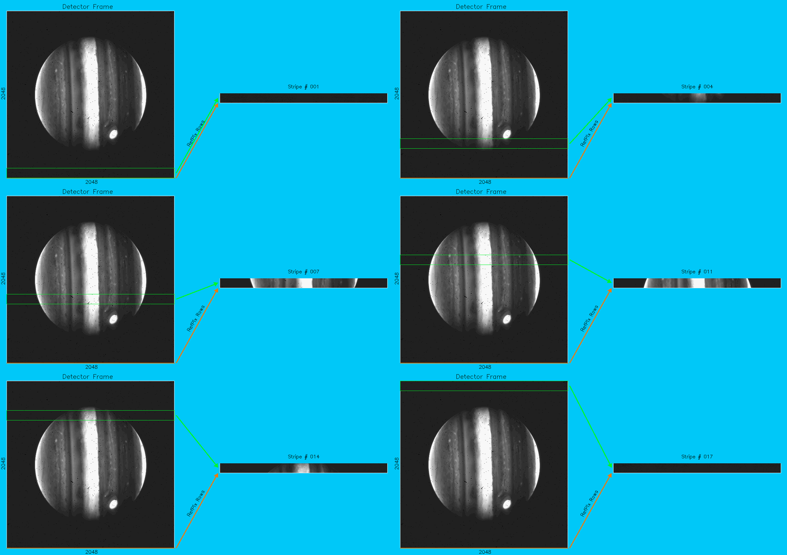
Right-click and open in a new tab or window to replay the animation.
Click on the figure for a larger view.
The animation above illustrates how the 17 superstripes of NIRCam's FULL_SUPSTP120 subarray are addressed during an exposure with # of integrations = 3. (A NIRCam F212N image of Jupiter was used as input to the simulation). The green box shows the position of the superstripe during each stripe integration; the red box shows the reference rows that are read just prior to the science pixel rows in the superstripe. Reference pixels appear white here. The smaller image at right shows the individual superstripe frames with reference rows and science rows combined.
Because reference pixels (shown as white in Figure 2) are interleaved with the science rows of the stripes, the Y dimension of such an image is larger than 2040. For the example shown, each of the 17 stripes of 120 rows has 2 reference pixel rows, so there are a total of 2074 rows in the image. During subsequent pipeline processing the reference rows are: (1) used to correct the science row data, (2) extracted and discarded in higher level FITS products. Level-2a products (e.g., _rate.fits) and their level-2b and level-3 derivatives (e.g., _cal.fits, _i2d.fits) have the science pixel stripes stitched together to produce normal full frame images.
Figure 2. An example level-1b (_uncal.fits) image resulting from a FULL_SUPSTP120 subarray exposure
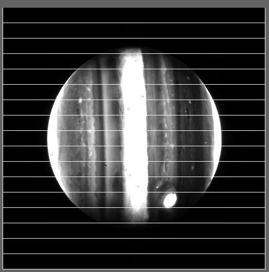
This figure illustrates how the 17 superstripes of a NIRCam's FULL_SUPSTP120 subarray exposure are initially organized in level-1 "_uncal.fits" files by the ground system.
NIRCam superstripe subarray properties
The basic properties of the 7 types of NIRCam superstripe subarrays are summarized in Table 2. The properties of the two comparable non-superstripe subarrays are given for comparison in parenthesis.
Table 2. Properties of NIRCam superstripe subarrays and those of the comparable normal subarrays
Subarray | Stripe frame | Bright limit increase (approximate) | |||||
|---|---|---|---|---|---|---|---|
| Stripe subarray (Comp. subarray) | nCols × nRows (science) | # of Stripes (nStripes) | nRows | RefPix rows | Frame time (s) | Brightness | Magnitudes |
(FULL) | 2040 × 2040 | 1 | n/a | n/a | 10.73677 | - | - |
| FULL_SUPSTP510 | 4 | 510 | 4 | 2.69861 | 3.98 | -1.5 | |
| FULL_SUPSTP120 | 17 | 120 | 2 | 0.64453 | 16.7 | -3.1 | |
| FULL_SUPSTP024 | 85 | 24 | 2 | 0.14149 | 75.9 | -4.7 | |
| FULL_SUPSTP008 | 255 | 8 | 1 | 0.05241 | 205 | -5.8 | |
| (SUB64P) | 64 × 64 | 1 | n/a | n/a | 0.05016 | - | - |
| SUB64P_SUPSTP32 | 2 | 32 | 0 | 0.02584 | 1.94 | -0.72 | |
| SUB64P_SUPSTP008 | 8 | 8 | 0 | 0.00760 | 6.60 | -2.1 | |
| SUB64P_SUPSTP002 | 64 | 8 * | 1 | 0.00152 * | 11.0 | -2.6 | |
* The SUB64P_SUPSTP002 subarray consists of interleaved single rows of reference pixels and science pixels. The first group in an integration begins 0.00304 s after the reset. The science row is then sampled 4 times every 0.00152 s per 64 × 8 frame within an exposure pattern group.
† Appropriate for extended sources, line emission, etc.
Sensitivity and saturation limits
The superstripe subarrays are supported in the ETC. As with any other observing mode, the ETC should be used to estimate expected sensitivity and bright limits in detail for all science programs.
Table 2 summarizes the approximate enhancements to bright limits for the superstripe subarrays relative to the bright limits for the comparable normal subarrays.
The noise properties for observations using superstripe subarrays is predicted to be very similar to observations using the comparable subarrays read out normally. However, it is critical to understand that the photon collection time per pixel for a superstripe exposure is diminished by a factor of (1 / # of Stripes) for the superstripe case. This is the reason superstripe exposures offer much higher bright limits, but the trade-off is that the exposure time per pixel, and therefore sensitivity, for the same exposure parameters is decreased commensurately. Table 3 provides a comparison of output from the ETC for 3 examples from the 7 available superstripe subarrays.
Table 3. Sensitivity and saturation limits for superstripe subarray exposures compared to a comparable FULL subarray exposure
| |
ETC output provided on the Reports panel (lower right in the ETC GUI) in the Results tab of that panel for a FULL subarray exposure (left), a FULL_SUPSTP510 exposure (middle), and a FULL_SUPSTP120 exposure (right). The exposure specification is the same for all 3 except for the subarray selection. Results that are consequentially different between the 3 are highlighted in yellow boxes. The large, orange-highlighted box at the bottom indicates ETC values that were added to better illustrate the effect of superstripe subarrays for all 3 nIR instruments. Differences of note are: Results panel (upper):
Instrument and Detector panel (lower):
| |
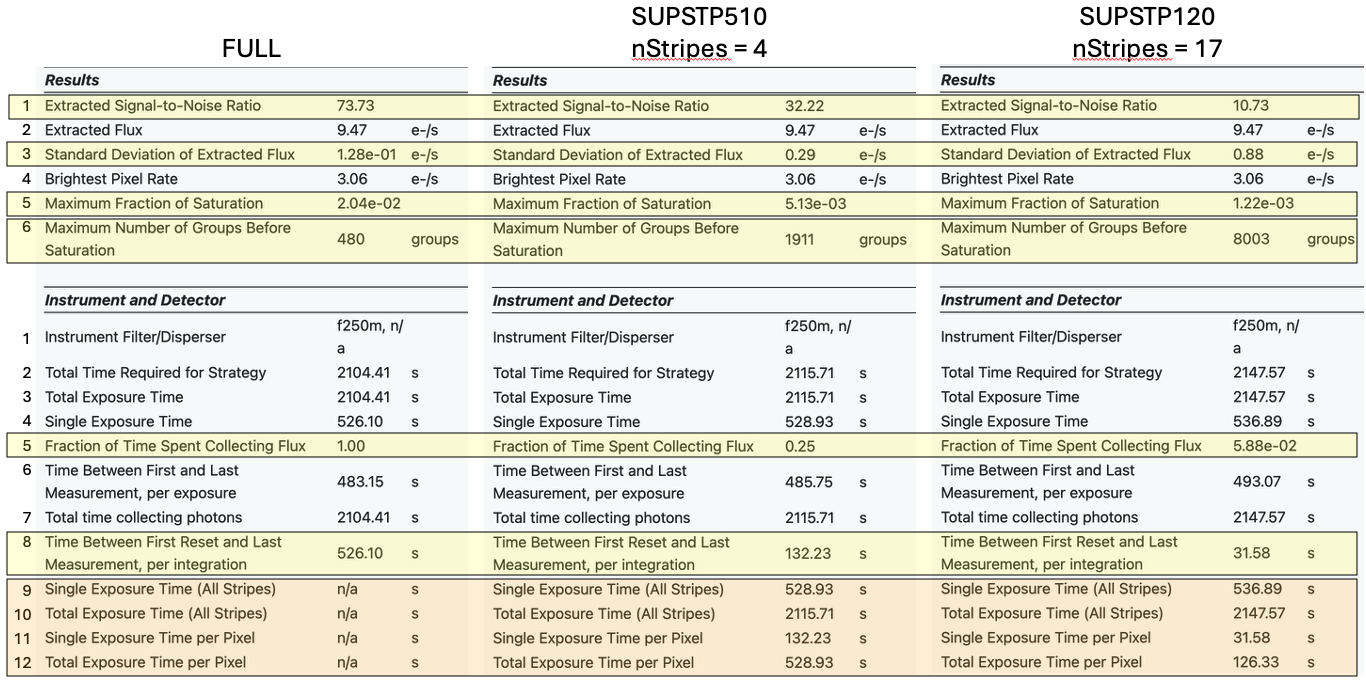
While Table 3 shows only two superstripe examples in comparison to a normal exposure, the comparison between comparably-sized normal subarrays and superstripe subarray is consistent. Namely, as the number of superstripes increases observing efficiency and sensitivity decrease, and bright limits increase, as a function of the number of superstripes.
Because superstripe exposures are less efficient than normal subarray exposures, they should only be used for observations requiring the enhanced bright limits they provide.
Timing considerations for time-variable sources
Because superstripe exposures complete integrations for each stripe (stripe-integrations) within the larger subarray area before cycling back to the first stripe for the next integration, the time sampling of the scene as a function of location on the detector is quite different than for normal readout. The exception to this would be for exposures with Groups / Int = 1. Taking FULL_SUPSTP120, Pattern = RAPID and Groups / Int = 10 as an example, the stripe integration for stripe 1 (rows 5–124) would end after 10 × 2.69861 s ≈ 27.0 s. The start of the integration for stripe 2 (rows 125–244) would occur at (10 + 1) × 2.69861 s ≈ 29.7 s ('+ 1' accounting for the reset frame at the end of stripe-integration 1), and take another ≈ 27.0 s to complete. For a normal FULL subarray RAPID integration with 2 groups, the entire frame would have been read out twice in 2 × 10.73677 ≈ 21.5 s. In the limiting case of a FULL_SUPSTP exposure with Groups / Int = 1, the timing would be nearly the same as for a normal FULL exposure, modulo only the time to read the extra reference rows and perform a reset after each stripe integration.
APT and ETC user interfaces
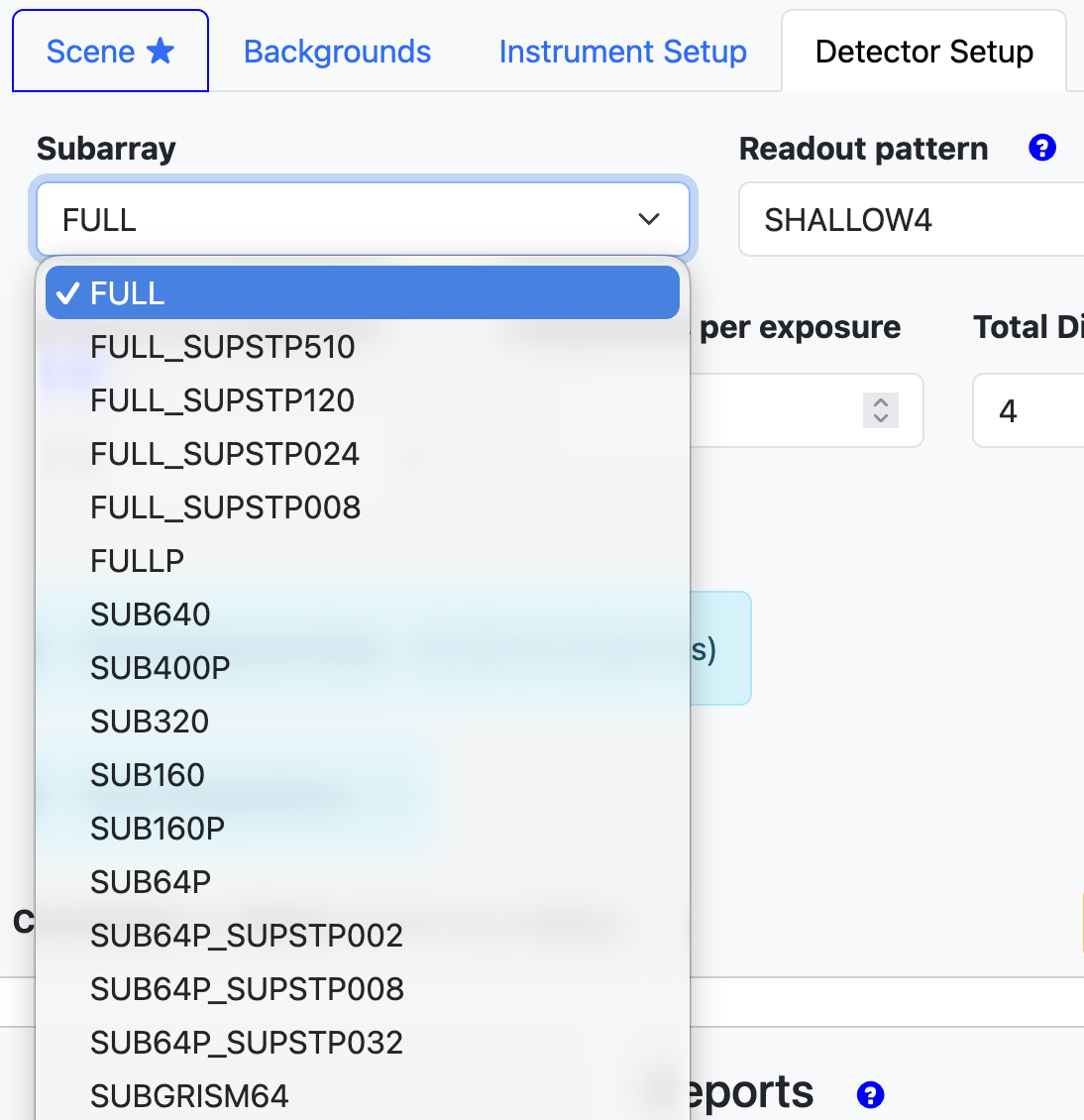
Updates to the APT and ETC interfaces for users are fairly minor, although there are changes to Total Exposure Time values when a superstripe subarray is used compared to when the comparable normal subarray is used, other exposure parameters being held constant. As mentioned above, the additional reset at the end of each stripe integration is primarily responsible for that increased time.
Table 4. APT and ETC subarray interfaces for superstripes
| APT Subarray selector* for superstripe subarrays for the time series (left) and imaging (right) templates | |||
|
|
|
|
ETC Subarray selectors for superstripe subarrays for the time-series (left) and imaging (right) templates. | |||
|
| ||
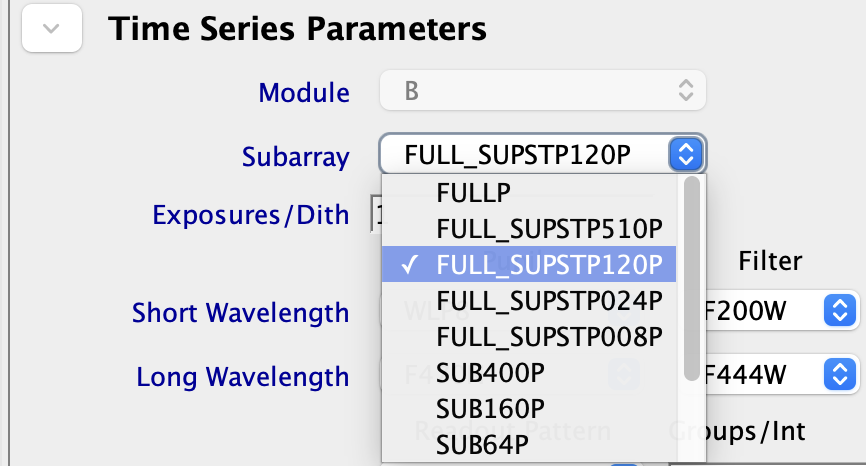
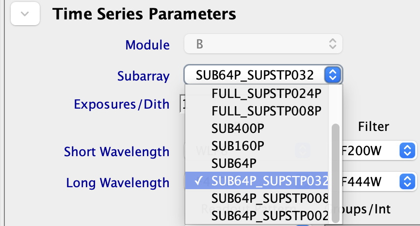
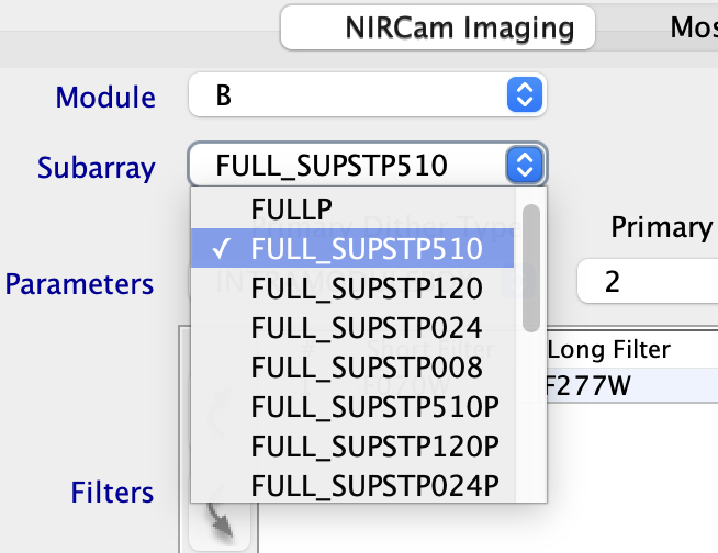
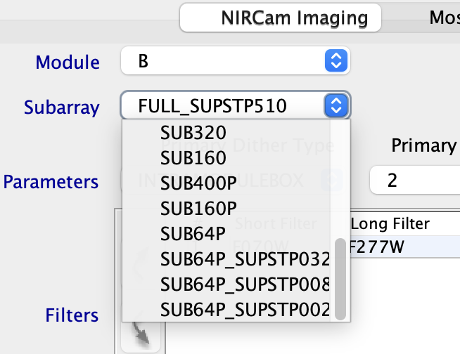
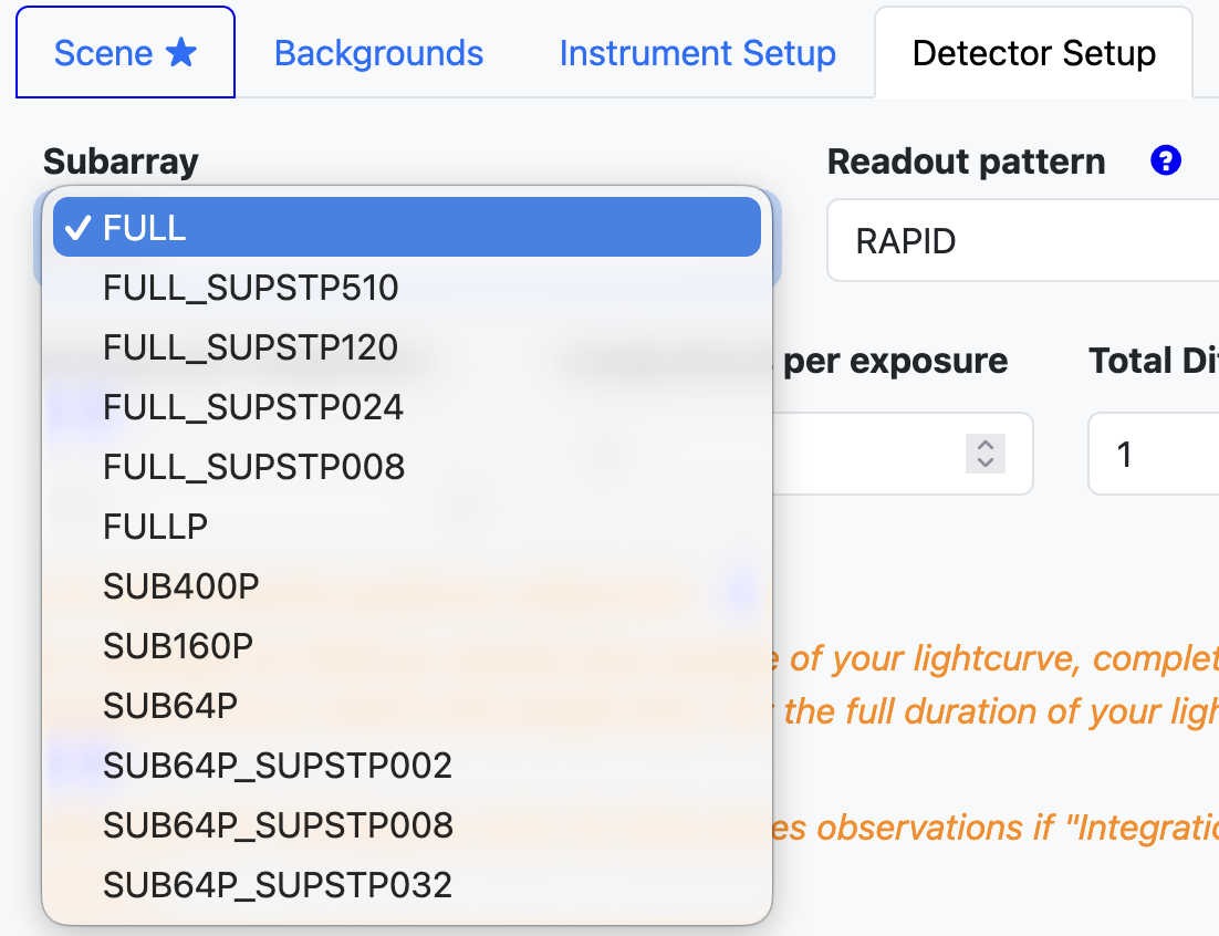
* The restricted height of the selector pull-down in APT limits the number of choices displayed at once, so 2 screenshots are provided for APT.