NIRSpec sensitivity estimates may be obtained using the JWST Exposure Time Calculator (ETC). Methods on how to do this and some best-estimates of limiting performance are available for users.

On this page

Information presented in the NIRSpec performance articles describes the best knowledge based on instrument component and flight modeling carried out on NIRSpec on-orbit data during the JWST instrument commissioning period. The best estimates of the on-orbit performance of all of JWST's instruments are incorporated into the JWST Exposure Time Calculators (ETC) starting with version 2.0. Additional calibration efforts will be undertaken during the JWST Cycle 1 observing period, and any further understanding and updates on instrument performance will be incorporated into the ETC and provided here as they become available.

Related NIRSpec on-orbit performance information can be found in these articles:

NIRSpec Sensitivity, the limiting flux sensitivity in a set of comparison ETC benchmark calculations.
NIRSpec Bright Source Limits, the brightest objects that may be observed using a given instrumental configuration.

The calculation method for sensitivity, transmission of the combined optical element and the efficiency of the detectors is discussed below.

From surface brightness to quantized units

The information shown here is meant as a guideline for the NIRSpec calculations in the linked subpages: NIRSpec Sensitivity and Bright Source Limits. The JWST Exposure Time Calculator (ETC) should be used to derive the best estimate of signal-to-noise and saturation limits for science sources of interest. A fuller discussion of signal-to-noise calculations is provided by Jakobsen et al. 2022.

The flux rate at the NIRSpec entrance aperture, $\begin{array}{l}S_\lambda^{ideal}\end{array}$ , is derived from the surface brightness of the astronomical source of interest $\begin{array}{l}(I_\lambda)\end{array}$ , the telescope collecting area (A) in cm² and the dimensionless combined transfer efficiency of the OTE (primary, secondary, tertiary, and fine steering mirrors) $\begin{array}{l}(\eta_{OTE}(\lambda))\end{array}$ .

(?)

$\begin{array}{l}\displaystyle S_{\lambda}^{ideal} = A \times \eta_{OTE}(\lambda)\times I_\lambda\end{array}$

where $\begin{array}{l}S_\lambda^{ideal}\end{array}$ is in units of photons/s/μm/pixel.

After the OTE, the flux is transferred through a specific instrument optics system.

Instrument optics systems are a crucial telescope component that can be described by one-dimensional (wavelength-dependent) efficiency curves (unity is perfect transmission). Each instrument/mode combination can have efficiency contributions from internal reflections and optical stops, filters, and dispersers. The actual focal plane flux rate is then:

(?)

$\begin{array}{l}\displaystyle S_{\lambda}^{\rm focal\, plane} = S_{\lambda}^{\rm ideal} \times \eta_{\rm optics}({\lambda}) \times \eta_{\rm filter}({\lambda}) \times \eta_{\rm disperser}({\lambda})\end{array}$

in units of photons/s/μm/pixel.

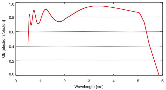
Faint sensitivity limits for a specific benchmark calculation case are described in the NIRSpec Sensitivity article. The signal to noise is derived from the number of incident photons measured by the end to end instrument, including the detector. This optical system transmission, $\begin{array}{l}S_\lambda\end{array}$ , follows from the above equation via a detector quantum efficiency function (QE; see the upper curve in Figure 1). The QE curve assumes a quantum yield (QY) of unity at all wavelengths (i.e., the efficiency of a detector at converting an incident photon to a measured electron is 1.0).

The optical transmission function is:

(?)

$\begin{array}{l}\displaystyle S_{\lambda} = S_{\lambda}^{\rm focal\, plane} \times {\rm QE}({\lambda})\end{array}$

in units of e^–/s/μm/pixel. The optical transmission is presented in Figure 2 for the NIRSpec grating-filter combinations using both the MOS internal optics throughput and the IFU internal optics throughput. Note that fixed slit (FS) spectroscopy shares the same optics as MOS.

Investigation of bright saturation limits for the NIRSpec detectors is described in the NIRSpec Bright Limits article. The calculations presented in the bright limit case measure the number of electrons that accumulate in the detector, based on the incident photons. In this case, the photon conversion efficiency (PCE) is used to present overall system efficiency of detecting electrons and filling the detector well. Calculation of the PCE uses the detector relative quantum efficiency (RQE), which is the QE multiplied by the quantum yield of the detector. At wavelengths shortward of 1.4 μm, a single incident photon can result in more than one electron measured on the detector. This results in a RQE greater than 1.0, as presented in the lower panel of Figure 1.

The PCE is:

(?)

$\begin{array}{l}\displaystyle PCE_{\lambda} = S_{\lambda}^{\rm focal\, plane} \times {\rm RQE}({\lambda})\end{array}$

in units of e^–/s/μm/pixel. The PCE is shown in Figure 3 for the MOS and the IFU internal optics throughputs.

The upper plot presents the NIRSpec quantum efficiency (QE) as a function of wavelength expressed in units of e^–/photon. Maximum efficiency is unity. The QE curve assumes a quantum yield (QY; efficiency of a detector at converting an incident photon to a measured electron) of unity at all wavelengths. The lower plot presents the relative quantum efficiency of the detector, RQE. This is the product of the QE and the actual quantum yield, which is not always unity. At wavelengths shortward of 1.4 μm the RQE is greater than 1.0 because an incident photon can result in more than one measured electron on the detector.

NIRSpec photon conversion efficiency (PCE) for a set of grating-filter combinations for the IFU observing mode. The colored lines present the on-orbit measured performance, while the colored regions present the pre-launch predicted performance. High-resolution grating data are presented in the top figure and medium resolution grating data are presented in the bottom figure. The medium resolution figure does not include data for the G140M/F100LP combination, which will be acquired during Cycle 1. (© Giardino et al. 2022.)

NIRSpec photon conversion efficiency (PCE) for a set of grating-filter combinations for the MOS observing mode. FS spectroscopy with NIRSpec uses the same optics as MOS. The colored lines present the on-orbit measured performance, while the colored regions present the pre-launch predicted performance. High-resolution grating data are presented in the top figure and medium resolution grating data are presented in the bottom figure. (© Giardino et al. 2022.)

References

Giardino, G., Bhatawdekar, R., Birkmann, S.M., et al. 2022, Proc. SPIE, 12180, 121800X (arXiv:2208.04876)
Optical throughput and sensitivity of the JWST NIRSpec

Jakobsen, P., Ferruit, P., Alves de Oliveira, C. et al. 2022, A&A, 661, A80
The Near-Infrared Spectrograph (NIRSpec) on the James Webb Space Telescope. I. Overview of the instrument and its capabilities

Pontoppidan, K. 2016, Proc of SPIE, 9910, 16
Pandeia: a multi-mission exposure time calculator for JWST and WFIRST

Latest updates	21 Nov 2022 Figures 2 and 3 replaced to show relative difference in PCE between pre-launch predictions and on-orbit performance
Originally published	23 Jan 2018

JWST User Documentation

NIRSpec Performance

From surface brightness to quantized units

References