ExoCTK Contamination Overlap Tool
The Contamination Overlap Tool is an observation planning tool that will provide the windows of time in which a given target may be observed and will also provide the levels of estimated contamination on the target's spectra due to neighboring sources in the field of view.
On this page
See also: JWST Position Angles, Ranges, and Offsets and JWST Observatory Coordinate System and Field of Regard
This tool is comprised of 2 calculators:
1. The Visibility Calculator, which predicts the aperture position angles (APAs) that a target can be observed in, and their corresponding visibility windows (up to Dec 31, 2024).
2. The Contamination Calculator, which determines the level of contamination on the target star from nearby point sources at each of these APAs.
These tools will aid the user in deciding which position angles to observe in, which will minimize potential contamination of target spectra from other point sources.
Both calculators are available on the ExoCTK website with the Visibility Calculator available for all JWST instruments: NIRCam, MIRI, NIRISS, NIRSpec, and FGS 1 and 2. The Contamination Calculator on the website is currently available for the NIRISS SOSS mode.
Results from observatory commissioning and Cycle 1 science programs indicate that distortion corrections need to be applied to precisely predict the final positioning of (contaminating) sources in the detector. The current version of the Contamination Overlap tool includes an empirical distortion correction based on commissioning and Early Release Science data for SOSS mode only.
Using the web interface
The Contamination Overlap tool can be found on the main page of the ExoCTK website under Observation Planning.

Words in bold are GUI menus/
panels or data software packages;
bold italics are buttons in GUI
tools or package parameters.


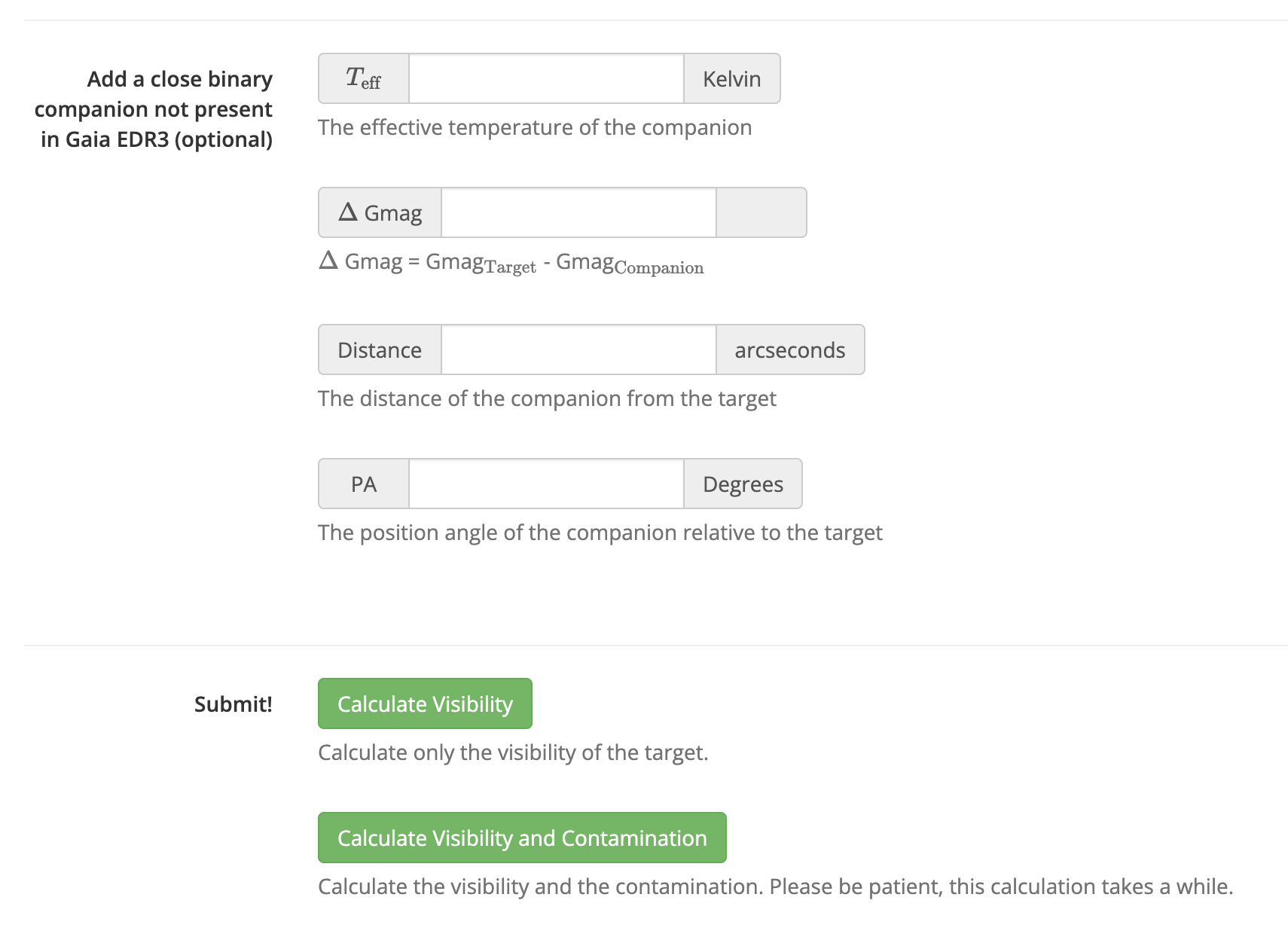
Once all of the fields are complete, the final step is to submit. As shown below, users can choose to calculate the visibility windows of the target, or its visibility and contamination. The "Visibility and Contamination" option will take a few seconds longer to run, as it generates a simulated field at every position angle of the instrument.
Visibility Calculator (available online)
After completing the steps above, the first result you should see is the Visibility Calculator result. An example of the Visibility Calculator output is shown below for target WASP-18b using the NIRISS instrument. The green lines represent the aperture position angles (APAs) in which the target can be observed, and the corresponding date (YYYY-MM-DD) the target can be observed in said angle. Hovering over a region of the bokeh plot on the website will show the maximum, nominal, and minimum aperture position angle, given the maximum boresight roll of the telescope for a given point, as well as the corresponding date. Users have the option to interact with the Visibility plot using the toolbar to the right of the plot which allows for zooming, panning, and saving the plot locally for future reference.

- Minimum V3 position angle (min_V3_PA), i.e., the angle of the entire JWST spacecraft with maximum clockwise boresight (V1) roll
- Maximum V3 position angle (max_V3_PA), i.e., the angle of the entire JWST spacecraft with maximum counterclockwise boresight (V1) roll
- Minimum aperture position angle (min_Aperture_PA), i.e., the angle of the JWST instrument with maximum clockwise boresight (V1) roll
- Maximum aperture position angle (max_Aperture_PA), i.e., the angle of the JWST instrument with maximum counterclockwise boresight (V1) roll
- Nominal aperture position angle (nom_Aperture_PA), i.e., the angle of the JWST instrument with no roll
- Gregorian date (YYYY-MM-DD HH:MM:SS)
- Modified Julian Date (MJD)
Below is an example .csv file for the WASP-18 NIRISS observation opened with Mac Numbers. The output .csv files can be opened with any data handling software.

Contamination Calculator for NIRISS SOSS mode (available online and locally)
If the user selects NIRISS - SOSS as their Instrument, there will be an option to calculate both the visibility and contamination on the target. The results page for this option will have another bokeh plot at the bottom showing the target's contamination as a function of aperture position angle and wavelength (in microns). The following is a screenshot taken from an example using WASP-18 b observed in NIRISS's SOSS mode. The following is an explication of the key features in the contamination plot:
- Top-left panel: The contamination for order 1 of the target trace. The contamination level is defined as the ratio of the extracted flux coming from all field stars over the extracted flux coming from the target star, using the proper extraction weighing function for the target trace. The deeper the color, the higher the degree of contamination, with white representing no contamination. The corresponding wavelength is in microns.
- Top-right panel: The % contamination of all spectral channels that are contaminated for order 1 at a level of at least 0.01 (green) or 0.001 (blue). 100% would indicate total contamination of the target trace (in every channel), 0% would indicate no contamination.
- Bottom-left panel: The contamination for order 2 of the target trace.
- Bottom-right panel: The % contamination of all spectral channels that are contaminated for order 2 at a level of at least 0.01 (green) or 0.001 (blue). 100% would indicate total contamination of the target trace (in every channel), 0% would indicate no contamination.
- The grey semi-transparent regions represent APAs where the target cannot be observed.
- The black crosshairs appear in both plots while hovering over the contamination images. The horizontal lines indicate the current position angle and the vertical lines indicate the wavelength.
Users can generate the plot below themselves with a local version of the ExoCTK package installed. For instructions on how to run the Contamination calculator locally, continue onto the next section.


Using the outputs
Once you have your outputs from Contamination Overlap, what do you do with them? In the Astronomer's Proposal Tool (APT), there is a field in the Observation panel under Special Requirements that allows users to specify the position angles that should be used for the observations. A demonstration of where this field can be found in APT is shown below. The figures below are of the APT version 27.2, using an example template of a NIRCam observation proposal.

Links
JWST Position Angles, Ranges, and Offsets
NIRISS Single Object Slitless Spectroscopy
MIRI Low Resolution Spectroscopy