JWST Coronagraphic Visibility Tool Help
The JWST Coronagraphic Visibility Tool (CVT) is a GUI-based target visibility tool for assessing target visibilities and available position angles versus time relative to the MIRI and NIRCam coronagraphic masks. Placement of up to 3 companions relative to the primary target can be entered for judging impacts from obscurations in the coronagraph fields of view.
On this page
See also: JWST Target Visibility Tools, JWST High-Contrast Imaging Roadmap
JWST observations have pointing constraints because the visibility of a target depends on the target's ecliptic latitude and time of observation. In addition, the allowed roll angle range depends on the solar elongation of the target's position at the time of observation. Allowed position angles (PAs) for a target can thus be a complicated function of time within each allowed visibility window. As a result, it can be difficult to:
- understand the possible orientations of a given target on the detector, especially in relation to any instrumental obscurations,
- determine the ideal roll angles and offsets for multi-roll observations, and
- determine the visibility of 2 or more targets that need to be observed simultaneously.
The JWST Coronagraph Visibility Tool (CVT) was created to address these issues and assist in planning MIRI and NIRCam coronagraphic programs prior to entering targets and observations into APT. The CVT will help you avoid problems in later APT scheduling and/or help diagnose scheduling errors that may crop up in APT. It is one of 2 tools available for investigating JWST target visibilities.
Note that the CVT is designed to provide quick illustrations of allowable observation orientations for a given target. While it approximates JWST’s pointing restrictions, it does not query the official JWST Proposal Constraint Generator (PCG) or check for guide star availability, as is done in APT. Therefore, CVT results should be treated as useful approximations that may differ from official APT constraints by a small amount (a degree or so).
Downloading and installing the CVT
The CVT has source code on GitHub at https://github.com/spacetelescope/jwst_coronagraph_visibility
Binary wheels for this package are distributed by PyPI. It can be installed for Python with pip:
pip install jwst-coronagraph-visibility
Specific details for using the target visibility tools are provided at the CVT help page. Please contact the JWST Help Desk with any questions regarding installation or usage.
If you're running macOS and want a double-clickable app:
- Download the double-clickable app archive (e.g., "jwst_coronagraph_visibility_tool_macos.zip") from https://github.com/spacetelescope/jwst_coronagraph_visibility/releases/latest
- Extract the ".zip" file to get the ".app" bundle
- Double-click the ".app" bundle
If you see a message warning you about opening an app from an unidentified developer, right-click (or control-left click) the icon and choose "Open". (This is a security feature of macOS.)
Using the coronagraphic visibility tool: a step by step example
See also: JWST Position Angles, Ranges, and Offsets.
Depending on how it was installed, you can open CVT from its app or from the command line. Double-clicking the app should open it, or from the command line enter
jwst-coronagraph-visibility-gui
After opening the program, a GUI should appear, as shown in Figure 1. (Initial startup may take a few seconds.) From here, everything is done through the GUI.

Words in bold are GUI menus/
panels or data software packages;
bold italics are buttons in GUI
tools or package parameters.
You can type coordinates into the RA and Dec boxes or use the target name resolver to get coordinates. To find a target, type the target name into the SIMBAD Target Resolver box and click Search. If SIMBAD is unable to find a match, the result "No object found for this identifier" will be displayed. If SIMBAD finds a match, the target’s SIMBAD ID, RA, and declination will be displayed. If SIMBAD cannot resolve a target, you may supply the RA and declination yourself (in decimal degrees).
The program also returns the ecliptic coordinates of the entered coordinate. The ecliptic latitude is of particular interest as the range of available position angles for a given target depends on it. Low ecliptic latitude targets may not be observable at certain angles—you will want to know this prior to specifying it for an APT observation.
Running the calculation
Once an RA and Dec are available in the tool, select the instrument and mask (defaults are "NIRCam channel A" and "NRCA2_MASK210R"), then click Update Plot to calculate the target’s visibility.
Figure 2 shows an example for the target HR 8799. The left plot shows the target's visibility windows. The red highlights on the solar elongation line indicate the valid windows. The blue tracks show the allowed position angles for the selected instrument and mask over those windows. The right panel shows the selected mask's field of view (red dashed line), where areas shaded in pink represent various obscurations due to hardware. These will change for different masks after the plot is updated.

The visibility plot shows the solar elongation for the target as a black line, with the observable portions (85°–135°) highlighted in red. This target has 2 valid windows over the year, read from the x-axis. For each red portion, the plot shows the range of allowed position angles in blue, read from the y-axis. ("Aperture PA" denotes the standard position angle, viz., the angle east from North to the instrument y-axis of the selected science instrument and mask.)
Note that although there are 2 good windows of visibility for this target, the range of allowed position angles for each of them is fairly restricted. Checking below the coordinate boxes in the control panel, you will see that the ecliptic latitude of HR 8799 is only 24.5°, which restricts the range of allowed angles available at any time for JWST.
You can do things like zoom in on any region of the plot, save the figure to a file, and reset to the original plot using Matplotlib's standard plot interactions, controlled by the icon bar at the lower left of the plot region. Hovering over each icon produces pop-up information about its functionality.
To plot the PA of the observatory V3 axis instead of the instrument/mask combination, click on the V3 PA button on the control panel and then Update Plot. The blue points will be replaced by purple points at the V3 PA values allowed for the observable periods.
Adding companions to the primary target
To plan observations of known companions, disks, or other structures, enable one of the Companions boxes by clicking on the check box in the left column. Specify the companion’s PA (in degrees E of N) and separation, Sep, (in arcseconds) from your primary target. A companion can be thought of as a binary star, an exoplanet, the location of a disk’s major or minor axis, or any sort of reference applicable to the astrophysical scene of interest. One can add up to 3 companions. The locations over time of the 1st, 2nd, and 3rd companions will be marked as tracks in the right panel plot with red, blue, and purple, respectively.
Before you update the plot, select or verify the instrument and coronagraphic mask that you’d like to use to observe the target using the drop-down menus. In this example, we select NIRCam and one of the wedge occulters.
Finally, click Update Plot again to refresh the plots. Figure 3 shows an example for HR 8799 in which we have plotted 3 companions to be observed with the NIRCam SWB mask.

You can now click on a blue point in the left visibility plot to select it; the corresponding companion points in time are marked on the right science detector panel in white. The north and east axes are also shown on the science frame as a solid red and yellow line, respectively. The default active field of view size for the selected mask and detector is also displayed on the science frame as a red dashed border. This is useful in scenarios where the astrophysical scene may exceed the aperture size.
You can zoom in on the plot using the plot controls at lower left. Also, when the cursor is within an active plot region, the cursor values appear at the lower right of the overall plot frame when the zoom controls are not active, so values can be seen directly (rather than reading them off the axes). The units on the left panel are degrees on the y-axis and days on the x-axis, referenced to January 1 of a generic year. (The pattern repeats from year to year.)
Use the zoom icon on the toolbar below the plots to enter zoom mode, which will let you enlarge the plot region of interest in either plot panel. Note that an indicator appears at lower right to indicate when the zoom mode is active. (Alternatively, one can select the pan and zoom feature, but the regular zoom is likely more appropriate for these plots.)
Note that each plot is cached, so you can use the forward and back arrow icons to navigate through previous plots. The home icon restores the original plot.
Alternatively, one can select a companion position in the right panel (click on a red, blue, or purple point) and see the corresponding position appear on the left visibility plot. The corresponding companion points are highlighted in white, and the corresponding PA is highlighted in white in the left panel.
Below the science panel, the separation (in arcsec) and angle on the detector (CCW relative to +y axis) are displayed for each white point. Figure 4 shows a particular observation date and roll angle for the HR 8799 system when all 3 companions are visible without obscuration.
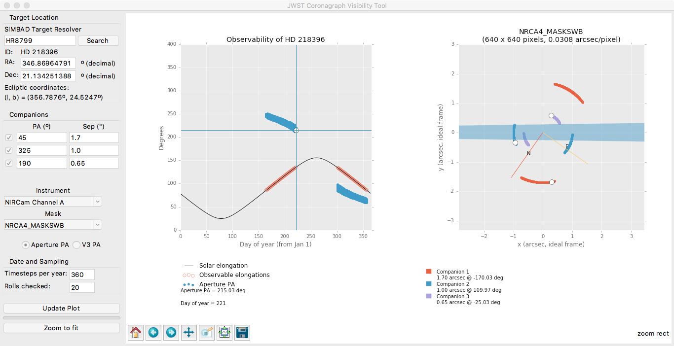
So far, this exercise has determined a time/angle (aperture PA of approximately 215°) when all 3 companions are nominally visible outside the obscuration of the mask. But for many coronagraphic applications, you may want to observe the target with a roll dither. Figure 5 shows what Figure 4 looks like when we zoom in on the visibility window in the left plot panel.
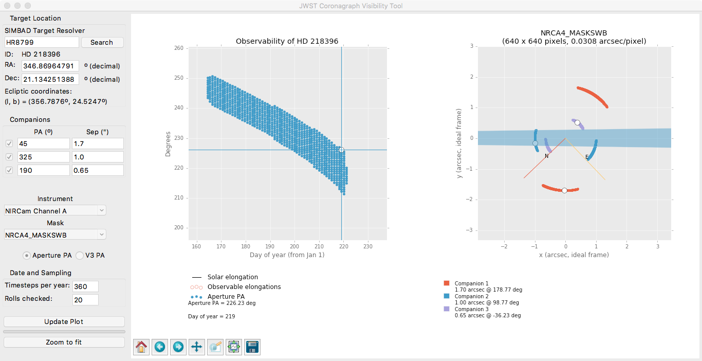
For this example, you will see that the companion on the blue track in the right panel rotates into the mask and becomes unobservable when the top of the blue range is selected in the left panel. You can use this sort of analysis to decide on how to restrict the size of the allowed roll offset to prevent this obscuration from happening, or investigate visibility in the other observing window to see if there is an alternative configuration that works better.

In Figure 6, we have now zoomed in on the first visibility window in the left plot and highlighted a time when all 3 companions are visible outside the wedge obscuration. However, 2 of the companions are very close to the mask, and once again, checking the availability for roll dithering shows problems. At this point, you will need to decide whether the former option is better, whether to include the small roll dither or not, and/or whether it would be more beneficial to make 2 observations of the field separated in time instead of using a roll dither.
Finally, for systems with other structure around the primary target, such as a disk with some known orientation on the sky, you can define a "companion" (or 2 diametrically opposed companions if desired) at the relevant position angle to act as a proxy for the disk structure's position angle versus time in the selected instrument and mask.
Saving plots
The rightmost icon in the plot control menu saves a file with the current plot view. The target name and instrument/mask information is encoded in the plot headers. However, the control panel (including any definitions of companions) is not saved. If needed, we suggest the option of performing a screen grab to save the desired display for your reference.
Checking visibility of PSF reference stars
The other important aspect of visibility for coronagraphic observers is the visibility of an appropriate reference star for point spread function (PSF) subtraction. In the vast majority of cases, the standard observation sequence includes an observation of the nominal science target and the PSF reference star in a contiguous, non-interruptible sequence, meaning that both objects need to be observable at the same time. Hence, once any restrictions on the observability of the science target are known, the CVT should be run on the potential PSF reference star or stars to verify that it's visible at the same time. For a PSF reference star, only the left panel (the visibility plot) is needed. (This can also be done using the General Target Visibility Tool (GTVT) since it does not require information about the coronagraphs.)
Final notes
The example above demonstrates the utility of looking at the details of potential coronagraphic observations prior to entering observations in APT. APT can provide accurate assessments of visibility windows and check such things as guide star availability for a particular time, but it is not optimized to provide assessments of how the NIRCam and/or MIRI masks impact the observability of known companions or disks. By checking such things within the CVT, you will be able to identify appropriate times and/or angles, and have good confidence that observations will be schedulable when their details are entered into the appropriate APT observation template(s). Alternatively, if the CVT shows that a particular target cannot be observed at the desired angle, it may be time to find a different target; at least you will have found this out prior to entering and trying to process a non-schedulable observation in APT.
The CVT, GTVT, and APT have been tested against each other for consistency. However, as stressed in the introduction, the CVT does not generate official pointing restrictions; you should consider the results as approximate and plan accordingly. For example, you should not rely on this tool to ensure that the orientation on the detector is accurate to within a degree of the reported angle or within a day of the beginning or end of the calculated visibility windows. This tool is not to be used for assessing the placement of any companion on a given pixel of the selected detector. It is for quick look and preliminary planning purposes only, but should result in a significant time savings for coronagraphic proposers.
Additional information on JWST’s pointing restrictions, and how those affect target visibility and available position angles are included in this page: JWST Position Angles, Ranges, and Offsets.